Analysis for joxm: using Cardelino-relax assignments
Davis J. McCarthy
Last updated: 2019-10-30
Checks: 7 0
Knit directory: fibroblast-clonality/
This reproducible R Markdown analysis was created with workflowr (version 1.4.0). The Checks tab describes the reproducibility checks that were applied when the results were created. The Past versions tab lists the development history.
Great! Since the R Markdown file has been committed to the Git repository, you know the exact version of the code that produced these results.
Great job! The global environment was empty. Objects defined in the global environment can affect the analysis in your R Markdown file in unknown ways. For reproduciblity it’s best to always run the code in an empty environment.
The command set.seed(20180807) was run prior to running the code in the R Markdown file. Setting a seed ensures that any results that rely on randomness, e.g. subsampling or permutations, are reproducible.
Great job! Recording the operating system, R version, and package versions is critical for reproducibility.
Nice! There were no cached chunks for this analysis, so you can be confident that you successfully produced the results during this run.
Great job! Using relative paths to the files within your workflowr project makes it easier to run your code on other machines.
Great! You are using Git for version control. Tracking code development and connecting the code version to the results is critical for reproducibility. The version displayed above was the version of the Git repository at the time these results were generated.
Note that you need to be careful to ensure that all relevant files for the analysis have been committed to Git prior to generating the results (you can use wflow_publish or wflow_git_commit). workflowr only checks the R Markdown file, but you know if there are other scripts or data files that it depends on. Below is the status of the Git repository when the results were generated:
Ignored files:
    Ignored:    .DS_Store
    Ignored:    .Rhistory
    Ignored:    .Rproj.user/
    Ignored:    .vscode/
    Ignored:    code/.DS_Store
    Ignored:    code/selection/.DS_Store
    Ignored:    code/selection/.Rhistory
    Ignored:    code/selection/figures/
    Ignored:    data/.DS_Store
    Ignored:    logs/
    Ignored:    src/.DS_Store
    Ignored:    src/Rmd/.Rhistory

Untracked files:
    Untracked:  .dockerignore
    Untracked:  .dropbox
    Untracked:  .snakemake/
    Untracked:  Rplots.pdf
    Untracked:  Snakefile_clonality
    Untracked:  Snakefile_somatic_calling
    Untracked:  analysis/.ipynb_checkpoints/
    Untracked:  analysis/assess_mutect2_fibro-ipsc_variant_calls.ipynb
    Untracked:  analysis/cardelino_fig1b.R
    Untracked:  analysis/cardelino_fig2b.R
    Untracked:  code/analysis_for_garx.Rmd
    Untracked:  code/selection/data/
    Untracked:  code/selection/fit-dist.nb
    Untracked:  code/selection/result-figure.R
    Untracked:  code/yuanhua/
    Untracked:  data/Melanoma-RegevGarraway-DFCI-scRNA-Seq/
    Untracked:  data/PRJNA485423/
    Untracked:  data/canopy/
    Untracked:  data/cell_assignment/
    Untracked:  data/cnv/
    Untracked:  data/de_analysis_FTv62/
    Untracked:  data/donor_info_070818.txt
    Untracked:  data/donor_info_core.csv
    Untracked:  data/donor_neutrality.tsv
    Untracked:  data/exome-point-mutations/
    Untracked:  data/fdr10.annot.txt.gz
    Untracked:  data/human_H_v5p2.rdata
    Untracked:  data/human_c2_v5p2.rdata
    Untracked:  data/human_c6_v5p2.rdata
    Untracked:  data/neg-bin-rsquared-petr.csv
    Untracked:  data/neutralitytestr-petr.tsv
    Untracked:  data/raw/
    Untracked:  data/sce_merged_donors_cardelino_donorid_all_qc_filt.rds
    Untracked:  data/sce_merged_donors_cardelino_donorid_all_with_qc_labels.rds
    Untracked:  data/sce_merged_donors_cardelino_donorid_unstim_qc_filt.rds
    Untracked:  data/sces/
    Untracked:  data/selection/
    Untracked:  data/simulations/
    Untracked:  data/variance_components/
    Untracked:  docs/figure/clone_prevalences_cardelino-relax.Rmd/
    Untracked:  figures/
    Untracked:  output/differential_expression/
    Untracked:  output/differential_expression_cardelino-relax/
    Untracked:  output/donor_specific/
    Untracked:  output/line_info.tsv
    Untracked:  output/nvars_by_category_by_donor.tsv
    Untracked:  output/nvars_by_category_by_line.tsv
    Untracked:  output/variance_components/
    Untracked:  qolg_BIC.pdf
    Untracked:  references/
    Untracked:  reports/
    Untracked:  src/Rmd/DE_pathways_FTv62_callset_clones_pairwise_vs_base.unst_cells.carderelax.Rmd
    Untracked:  src/Rmd/Rplots.pdf
    Untracked:  src/Rmd/cell_assignment_cardelino-relax_template.Rmd
    Untracked:  tree.txt
Note that any generated files, e.g. HTML, png, CSS, etc., are not included in this status report because it is ok for generated content to have uncommitted changes.
These are the previous versions of the R Markdown and HTML files. If you’ve configured a remote Git repository (see ?wflow_git_remote), click on the hyperlinks in the table below to view them.
| File | Version | Author | Date | Message |
|---|---|---|---|---|
| Rmd | f2e01ef | Davis McCarthy | 2019-10-30 | Couple of typo fixes |
| Rmd | 550176f | Davis McCarthy | 2019-10-30 | Updating analysis to reflect accepted ms |
Load libraries and data
knitr::opts_chunk$set(echo = TRUE, warning = FALSE, message = FALSE,
                      fig.height = 10, fig.width = 14)
dir.create("figures/donor_specific", showWarnings = FALSE, recursive = TRUE)
library(tidyverse)
library(scater)
library(ggridges)
library(GenomicRanges)
library(RColorBrewer)
library(edgeR)
library(ggrepel)
library(rlang)
library(limma)
library(org.Hs.eg.db)
library(ggforce)
library(cardelino)
library(cowplot)
library(IHW)
library(viridis)
library(ggthemes)
library(superheat)
options(stringsAsFactors = FALSE)
Load MSigDB gene sets.
Load VEP consequence information.
vep_best <- read_tsv("data/exome-point-mutations/high-vs-low-exomes.v62.ft.alldonors-filt_lenient.all_filt_sites.vep_most_severe_csq.txt")
colnames(vep_best)[1] <- "Uploaded_variation"
## deduplicate dataframe
vep_best <- vep_best[!duplicated(vep_best[["Uploaded_variation"]]),]
Load somatic variant sites from whole-exome sequencing data.
exome_sites <- read_tsv("data/exome-point-mutations/high-vs-low-exomes.v62.ft.filt_lenient-alldonors.txt.gz",
    col_types = "ciccdcciiiiccccccccddcdcll", comment = "#",
    col_names = TRUE)
exome_sites <- dplyr::mutate(
    exome_sites,
    chrom = paste0("chr", gsub("chr", "", chrom)),
    var_id = paste0(chrom, ":", pos, "_", ref, "_", alt))
## deduplicate sites list
exome_sites <- exome_sites[!duplicated(exome_sites[["var_id"]]),]
Add consequences to exome sites.
vep_best[["var_id"]] <- paste0("chr", vep_best[["Uploaded_variation"]])
exome_sites <- inner_join(exome_sites,
                           vep_best[, c("var_id", "Location", "Consequence")],
                           by = "var_id")
Load cell-clone assignment results for this donor.
cell_assign_joxm <- readRDS(file.path("data/cell_assignment",
        paste0("cardelino_results_carderelax.joxm.filt_lenient.cell_coverage_sites.rds")))
Load SCE objects.
params <- list()
params$callset <- "filt_lenient.cell_coverage_sites"
fls <- list.files("data/sces")
fls <- fls[grepl(paste0("carderelax.", params$callset), fls)]
donors <- gsub(".*ce_([a-z]+)_with_clone_assignments_carderelax.*", "\\1", fls)

sce_unst_list <- list()
for (don in donors) {
    sce_unst_list[[don]] <- readRDS(file.path("data/sces",
        paste0("sce_", don, "_with_clone_assignments_carderelax.",
               params$callset, ".rds")))
    cat(paste("reading", don, ":   ", ncol(sce_unst_list[[don]]),
              "unstimulated cells.\n"))
}
reading euts : 79 unstimulated cells.
reading fawm : 53 unstimulated cells.
reading feec : 75 unstimulated cells.
reading fikt : 39 unstimulated cells.
reading garx : 70 unstimulated cells.
reading gesg : 105 unstimulated cells.
reading heja : 50 unstimulated cells.
reading hipn : 62 unstimulated cells.
reading ieki : 58 unstimulated cells.
reading joxm : 79 unstimulated cells.
reading kuco : 48 unstimulated cells.
reading laey : 55 unstimulated cells.
reading lexy : 63 unstimulated cells.
reading naju : 44 unstimulated cells.
reading nusw : 60 unstimulated cells.
reading oaaz : 38 unstimulated cells.
reading oilg : 90 unstimulated cells.
reading pipw : 107 unstimulated cells.
reading puie : 41 unstimulated cells.
reading qayj : 97 unstimulated cells.
reading qolg : 36 unstimulated cells.
reading qonc : 58 unstimulated cells.
reading rozh : 91 unstimulated cells.
reading sehl : 30 unstimulated cells.
reading ualf : 89 unstimulated cells.
reading vass : 37 unstimulated cells.
reading vils : 37 unstimulated cells.
reading vuna : 71 unstimulated cells.
reading wahn : 82 unstimulated cells.
reading wetu : 77 unstimulated cells.
reading xugn : 35 unstimulated cells.
reading zoxy : 88 unstimulated cells.assignments_lst <- list()
for (don in donors) {
assignments_lst[[don]] <- as_tibble(
colData(sce_unst_list[[don]])[,
c("donor_short_id", "highest_prob",
"assigned", "total_features",
"total_counts_endogenous", "num_processed")])
}
assignments <- do.call("rbind", assignments_lst)Load the SCE object for joxm.
sce_joxm <- readRDS("data/sces/sce_joxm_with_clone_assignments_carderelax.filt_lenient.cell_coverage_sites.rds")
sce_joxm
class: SingleCellExperiment
dim: 13225 79
metadata(1): log.exprs.offset
assays(2): counts logcounts
rownames(13225): ENSG00000000003_TSPAN6 ENSG00000000419_DPM1 ...
ERCC-00170_NA ERCC-00171_NA
rowData names(11): ensembl_transcript_id ensembl_gene_id ...
is_feature_control high_var_gene
colnames(79): 22259_2#169 22259_2#173 ... 22666_2#70 22666_2#71
colData names(128): salmon_version samp_type ... nvars_cloneid
clone_apk2
reducedDimNames(0):
spikeNames(1): ERCCWe can check cell assignments for this donor.
    clone1     clone2     clone3 unassigned
        46         25          7          1
Load DE results (obtained using the edgeR quasi-likelihood F test and the camera method from the limma package).
Tree and probability heatmap
We can plot the clonal tree inferred with Canopy for this donor along with the cell-clone assignment results from cardelino.
Plot tree (updated tree output by Cardelino) with assignment probability matrix.
fig_tree <- plot_tree(cell_assign_joxm$full_tree, orient = "v") +
    xlab("Clonal tree") +
    cardelino:::heatmap.theme(size = 16) +
    theme(axis.text.x = element_blank(), axis.title.y = element_text(size = 20))

prob_to_plot <- cell_assign_joxm$prob_mat[
    colnames(sce_joxm)[sce_joxm$well_condition == "unstimulated"], ]
hc <- hclust(dist(prob_to_plot))

clone_ids <- colnames(prob_to_plot)
clone_frac <- colMeans(prob_to_plot[matrixStats::rowMaxs(prob_to_plot) > 0.5,])
clone_perc <- paste0(clone_ids, ": ",
                          round(clone_frac*100, digits = 1), "%")

colnames(prob_to_plot) <- clone_perc
nba.m <- as_data_frame(prob_to_plot[hc$order,]) %>%
    dplyr::mutate(cell = rownames(prob_to_plot[hc$order,])) %>%
    gather(key = "clone", value = "prob", -cell)
nba.m <- dplyr::mutate(nba.m, cell = factor(
    cell, levels = rownames(prob_to_plot[hc$order,])))
fig_assign <- ggplot(nba.m, aes(clone, cell, fill = prob)) +
    geom_tile(show.legend = TRUE) +
    # scale_fill_gradient(low = "white", high = "firebrick4",
    #                     name = "posterior probability of assignment") +
    scico::scale_fill_scico(palette = "oleron", direction = 1) +
    ylab(paste("Single cells")) +
    cardelino:::heatmap.theme(size = 16) + #cardelino:::pub.theme() +
    theme(axis.title.y = element_text(size = 20), legend.position = "bottom",
          legend.text = element_text(size = 12), legend.key.size = unit(0.05, "npc"))

plot_grid(fig_tree, fig_assign, nrow = 2, rel_heights = c(0.46, 0.52))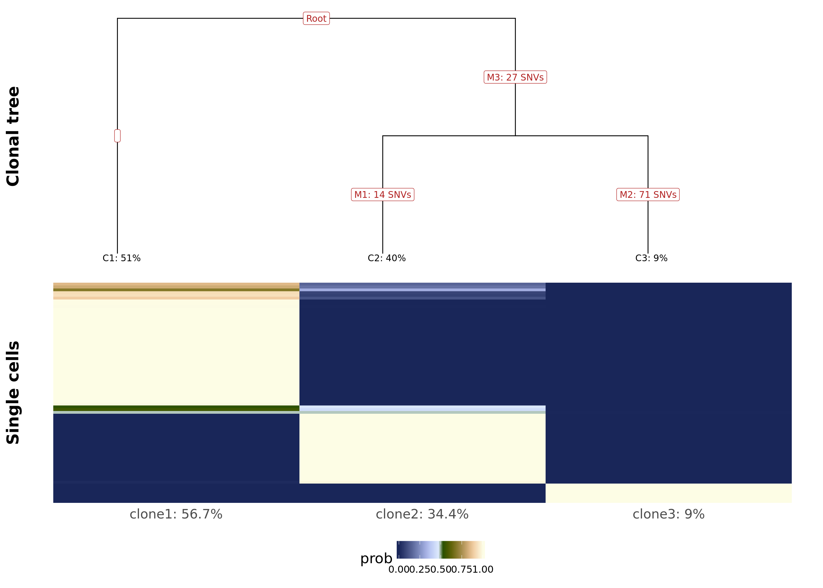
ggsave("figures/donor_specific/carderelax_joxm_tree_probmat.png", height = 10, width = 7.5)
ggsave("figures/donor_specific/carderelax_joxm_tree_probmat.pdf", height = 10, width = 7.5)
ggsave("figures/donor_specific/carderelax_joxm_tree_probmat.svg", height = 10, width = 7.5)

ggsave("figures/donor_specific/carderelax_joxm_tree_probmat_wide.png", height = 9, width = 10)
ggsave("figures/donor_specific/carderelax_joxm_tree_probmat_wide.pdf", height = 9, width = 10)
ggsave("figures/donor_specific/carderelax_joxm_tree_probmat_wide.svg", height = 9, width = 10)
Analysis of direct effects of variants on gene expression
Load SCE object and cell assignment results.
First, plot the VEP consequences of somatic variants in this donor used to infer the clonal tree.
joxm_config <- as_data_frame(cell_assign_joxm$full_tree$Z)
joxm_config[["var_id"]] <- rownames(cell_assign_joxm$full_tree$Z)
exome_sites_joxm <- inner_join(exome_sites, joxm_config)
exome_sites_joxm[["clone_presence"]] <- ""
for (cln in colnames(cell_assign_joxm$full_tree$Z)[-1]) {
    exome_sites_joxm[["clone_presence"]][
        as.logical(exome_sites_joxm[[cln]])] <- paste(
            exome_sites_joxm[["clone_presence"]][
                as.logical(exome_sites_joxm[[cln]])], cln, sep = "&")
}
exome_sites_joxm[["clone_presence"]] <- gsub("^&", "",
                                        exome_sites_joxm[["clone_presence"]])

exome_sites_joxm %>% group_by(Consequence, clone_presence) %>%
    summarise(n_vars = n()) %>%
ggplot(aes(x = n_vars, y = reorder(Consequence, n_vars, max),
       colour = reorder(Consequence, n_vars, max))) +
    geom_point(size = 5) +
    geom_segment(aes(x = 0, y = Consequence, xend = n_vars, yend = Consequence)) +
    facet_wrap(~clone_presence) +
#    scale_color_brewer(palette = "Set2") +
    scale_color_manual(values = colorRampPalette(brewer.pal(8, "Accent"))(12)) +
    guides(colour = FALSE) +
    ggtitle("joxm clone tagging variants by consequence class") +
    xlab("number of variants") + ylab("consequence") +
    theme_bw(16)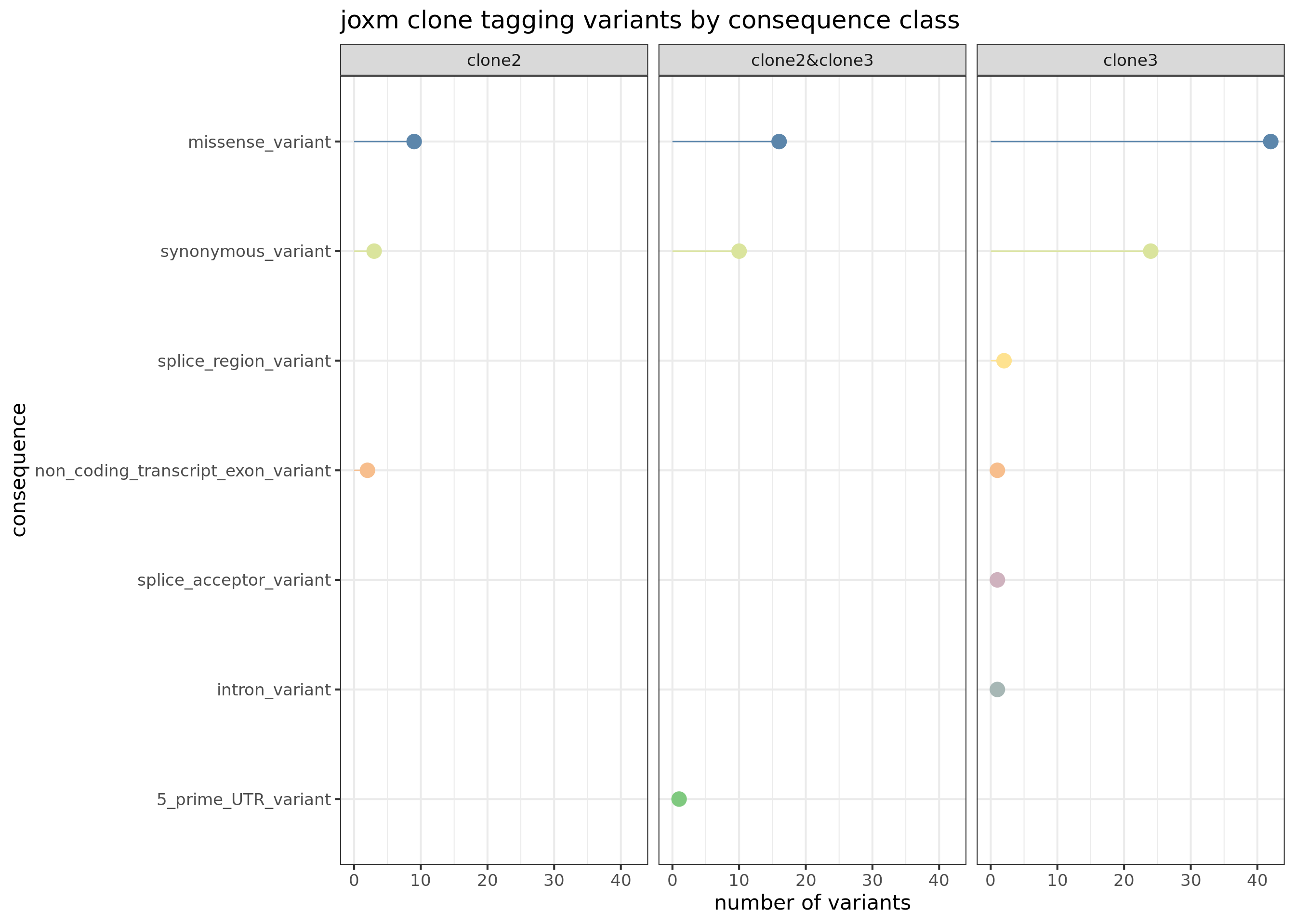
Look at expression of genes with mutations.
Organise data for analysis.
## filter out any remaining ERCC genes
sce_joxm <- sce_joxm[!rowData(sce_joxm)$is_feature_control,]
sce_joxm_gr <- makeGRangesFromDataFrame(rowData(sce_joxm),
                                   start.field = "start_position",
                                   end.field = "end_position",
                                   keep.extra.columns = TRUE)
exome_sites_joxm[["chrom"]] <- gsub("chr", "", exome_sites_joxm[["chrom"]])
exome_sites_joxm_gr <- makeGRangesFromDataFrame(exome_sites_joxm,
                                   start.field = "pos",
                                   end.field = "pos",
                                   keep.extra.columns = TRUE)
# find overlaps
ov_joxm <- findOverlaps(sce_joxm_gr, exome_sites_joxm_gr)
tmp_cols <- colnames(mcols(exome_sites_joxm_gr))
tmp_cols <- tmp_cols[grepl("clone", tmp_cols)]
tmp_cols <- c("Consequence", tmp_cols, "var_id")
mut_genes_exprs_joxm <- logcounts(sce_joxm)[queryHits(ov_joxm),]
mut_genes_df_joxm <- as_data_frame(mut_genes_exprs_joxm)
mut_genes_df_joxm[["gene"]] <- rownames(mut_genes_exprs_joxm)
mut_genes_df_joxm <- bind_cols(mut_genes_df_joxm,
                          as_data_frame(
                              exome_sites_joxm_gr[
                                  subjectHits(ov_joxm)])[, tmp_cols]
)
DE comparing mutated clone to all other clones
Get DE results comparing mutated clone to all unmutated clones.
cell_assign_list <- list()
for (don in donors) {
    cell_assign_list[[don]] <- readRDS(file.path("data/cell_assignment",
        paste0("cardelino_results.", don, ".", params$callset, ".rds")))
    cat(paste("reading", don, "\n"))
}
reading euts
reading fawm
reading feec
reading fikt
reading garx
reading gesg
reading heja
reading hipn
reading ieki
reading joxm
reading kuco
reading laey
reading lexy
reading naju
reading nusw
reading oaaz
reading oilg
reading pipw
reading puie
reading qayj
reading qolg
reading qonc
reading rozh
reading sehl
reading ualf
reading vass
reading vils
reading vuna
reading wahn
reading wetu
reading xugn
reading zoxy get_sites_by_donor <- function(sites_df, sce_list, assign_list) {
if (!identical(sort(names(sce_list)), sort(names(assign_list))))
stop("donors do not match between sce_list and assign_list.")
sites_by_donor <- list()
for (don in names(sce_list)) {
config <- as_data_frame(assign_list[[don]]$tree$Z)
config[["var_id"]] <- rownames(assign_list[[don]]$tree$Z)
sites_donor <- inner_join(sites_df, config)
sites_donor[["clone_presence"]] <- ""
for (cln in colnames(assign_list[[don]]$tree$Z)[-1]) {
sites_donor[["clone_presence"]][
as.logical(sites_donor[[cln]])] <- paste(
sites_donor[["clone_presence"]][
as.logical(sites_donor[[cln]])], cln, sep = "&")
}
sites_donor[["clone_presence"]] <- gsub("^&", "",
sites_donor[["clone_presence"]])
## drop config columns as these won't match up between donors
keep_cols <- grep("^clone[0-9]$", colnames(sites_donor), invert = TRUE)
sites_by_donor[[don]] <- sites_donor[, keep_cols]
}
do.call("bind_rows", sites_by_donor)
}
sites_by_donor <- get_sites_by_donor(exome_sites, sce_unst_list, cell_assign_list)
sites_by_donor_gr <- makeGRangesFromDataFrame(sites_by_donor,
start.field = "pos",
end.field = "pos",
keep.extra.columns = TRUE)
## run DE for mutated cells vs unmutated cells using existing DE results
## filter out any remaining ERCC genes
for (don in names(de_res[["sce_list_unst"]]))
de_res[["sce_list_unst"]][[don]] <- de_res[["sce_list_unst"]][[don]][
!rowData(de_res[["sce_list_unst"]][[don]])$is_feature_control,]
sce_de_list_gr <- list()
for (don in names(de_res[["sce_list_unst"]])) {
sce_de_list_gr[[don]] <- makeGRangesFromDataFrame(
rowData(de_res[["sce_list_unst"]][[don]]),
start.field = "start_position",
end.field = "end_position",
keep.extra.columns = TRUE)
seqlevelsStyle(sce_de_list_gr[[don]]) <- "UCSC"
}
mut_genes_df_allcells_list <- list()
for (don in names(de_res[["sce_list_unst"]])) {
cat("working on ", don, "\n")
sites_tmp <- sites_by_donor_gr[sites_by_donor_gr$donor_short_id == don]
ov_tmp <- findOverlaps(sce_de_list_gr[[don]], sites_tmp)
sce_tmp <- de_res[["sce_list_unst"]][[don]][queryHits(ov_tmp),]
sites_tmp <- sites_tmp[subjectHits(ov_tmp)]
sites_tmp$gene <- rownames(sce_tmp)
dge_tmp <- de_res[["dge_list"]][[don]]
dge_tmp <- dge_tmp[intersect(rownames(dge_tmp), sites_tmp$gene),]
base_design <- dge_tmp$design[, !grepl("assigned", colnames(dge_tmp$design))]
de_tbl_tmp <- data.frame(donor = don,
gene = sites_tmp$gene,
hgnc_symbol = gsub(".*_", "", sites_tmp$gene),
ensembl_gene_id = gsub("_.*", "", sites_tmp$gene),
var_id = sites_tmp$var_id,
location = sites_tmp$Location,
consequence = sites_tmp$Consequence,
clone_presence = sites_tmp$clone_presence,
logFC = NA, logCPM = NA, F = NA, PValue = NA,
comment = "")
for (i in seq_len(length(sites_tmp))) {
clones_tmp <- strsplit(sites_tmp$clone_presence[i], split = "&")[[1]]
mutatedclone <- as.numeric(sce_tmp$assigned %in% clones_tmp)
dsgn_tmp <- cbind(base_design, data.frame(mutatedclone))
if (sites_tmp$gene[i] %in% rownames(dge_tmp) && is.fullrank(dsgn_tmp)) {
qlfit_tmp <- glmQLFit(dge_tmp[sites_tmp$gene[i],], dsgn_tmp)
de_tmp <- glmQLFTest(qlfit_tmp, coef = ncol(dsgn_tmp))
de_tbl_tmp$logFC[i] <- de_tmp$table$logFC
de_tbl_tmp$logCPM[i] <- de_tmp$table$logCPM
de_tbl_tmp$F[i] <- de_tmp$table$F
de_tbl_tmp$PValue[i] <- de_tmp$table$PValue
}
if (!(sites_tmp$gene[i] %in% rownames(dge_tmp)))
de_tbl_tmp$comment[i] <- "gene did not pass DE filters"
if (!is.fullrank(dsgn_tmp))
de_tbl_tmp$comment[i] <- "insufficient cells assigned to clone"
}
mut_genes_df_allcells_list[[don]] <- de_tbl_tmp
}working on euts
working on fawm
working on feec
working on fikt
working on garx
working on gesg
working on heja
working on hipn
working on ieki
working on joxm
working on kuco
working on laey
working on lexy
working on naju
working on nusw
working on oaaz
working on oilg
working on pipw
working on puie
working on qayj
working on qolg
working on qonc
working on rozh
working on sehl
working on ualf
working on vass
working on vuna
working on wahn
working on wetu
working on xugn
working on zoxy mut_genes_df_allcells <- do.call("bind_rows", mut_genes_df_allcells_list)
## add FDRs for genes tested here for DE
ihw_res_all <- ihw(PValue ~ logCPM, data = mut_genes_df_allcells, alpha = 0.2)
mut_genes_df_allcells$FDR <- adj_pvalues(ihw_res_all)
## add simplified consequence categories
mut_genes_df_allcells$consequence_simplified <-
mut_genes_df_allcells$consequence
mut_genes_df_allcells$consequence_simplified[
mut_genes_df_allcells$consequence_simplified %in%
c("stop_retained_variant", "start_lost", "stop_lost", "stop_gained")] <- "nonsense"
mut_genes_df_allcells$consequence_simplified[
mut_genes_df_allcells$consequence_simplified %in%
c("splice_donor_variant", "splice_acceptor_variant", "splice_region_variant")] <- "splicing"
# table(mut_genes_df_allcells$consequence_simplified)
# dplyr::arrange(mut_genes_df_allcells, FDR) %>% dplyr::select(-location) %>% head(n = 20)For just the donor joxm.
tmp4 <- mut_genes_df_allcells %>%
    dplyr::filter(!is.na(logFC), donor == "joxm") %>%
    group_by(consequence_simplified) %>%
    summarise(med = median(logFC, na.rm = TRUE),
              nvars = n())
tmp4
# A tibble: 6 x 3
consequence_simplified med nvars
<chr> <dbl> <int>
1 5_prime_UTR_variant 1.02 1
2 intron_variant -0.627 2
3 missense_variant 0.266 70
4 non_coding_transcript_exon_variant 0.501 3
5 splicing -1.78 3
6 synonymous_variant 0.0835 36df_to_plot <- mut_genes_df_allcells %>%
dplyr::filter(!is.na(logFC), donor == "joxm") %>%
dplyr::mutate(
FDR = p.adjust(PValue, method = "BH"),
consequence_simplified = factor(
consequence_simplified,
levels(as.factor(consequence_simplified))[order(tmp4[["med"]])]),
de = ifelse(FDR < 0.2, "FDR < 0.2", "FDR > 0.2"))
df_to_plot %>%
dplyr::select(gene, hgnc_symbol, consequence, clone_presence, logFC,
F, FDR, PValue, ) %>%
dplyr::arrange(FDR) %>% head(n = 20) gene hgnc_symbol consequence
1 ENSG00000084764_MAPRE3 MAPRE3 missense_variant
2 ENSG00000108821_COL1A1 COL1A1 splice_region_variant
3 ENSG00000108821_COL1A1 COL1A1 splice_acceptor_variant
4 ENSG00000101407_TTI1 TTI1 synonymous_variant
5 ENSG00000101407_TTI1 TTI1 synonymous_variant
6 ENSG00000129295_LRRC6 LRRC6 missense_variant
7 ENSG00000070476_ZXDC ZXDC synonymous_variant
8 ENSG00000130881_LRP3 LRP3 synonymous_variant
9 ENSG00000130881_LRP3 LRP3 missense_variant
10 ENSG00000149090_PAMR1 PAMR1 missense_variant
11 ENSG00000171988_JMJD1C JMJD1C missense_variant
12 ENSG00000120910_PPP3CC PPP3CC missense_variant
13 ENSG00000120910_PPP3CC PPP3CC missense_variant
14 ENSG00000148634_HERC4 HERC4 missense_variant
15 ENSG00000113739_STC2 STC2 missense_variant
16 ENSG00000113739_STC2 STC2 synonymous_variant
17 ENSG00000164733_CTSB CTSB missense_variant
18 ENSG00000152104_PTPN14 PTPN14 missense_variant
19 ENSG00000107104_KANK1 KANK1 synonymous_variant
20 ENSG00000173933_RBM4 RBM4 missense_variant
clone_presence logFC F FDR PValue
1 clone3 3.8852622 23.551694 0.0006174704 6.836602e-06
2 clone3 -1.7755752 21.389937 0.0006174704 1.610792e-05
3 clone3 -1.7755752 21.389937 0.0006174704 1.610792e-05
4 clone3 -3.6592117 9.544347 0.0562436492 2.934451e-03
5 clone3 -3.6592117 9.544347 0.0562436492 2.934451e-03
6 clone3 4.1091706 10.394705 0.0562436492 2.146039e-03
7 clone2&clone3 1.7671121 9.083986 0.0664002981 4.041757e-03
8 clone3 -4.3468332 7.001221 0.1299831952 1.017260e-02
9 clone3 -4.3468332 7.001221 0.1299831952 1.017260e-02
10 clone2 1.6050652 6.297424 0.1642661344 1.434150e-02
11 clone3 -4.6591571 6.121515 0.1642661344 1.571241e-02
12 clone3 -3.8189782 5.637699 0.1663081972 2.024622e-02
13 clone3 -3.8189782 5.637699 0.1663081972 2.024622e-02
14 clone2 0.9119639 5.671353 0.1663081972 1.988993e-02
15 clone3 -2.0906592 5.350110 0.1694907959 2.358133e-02
16 clone3 -2.0906592 5.350110 0.1694907959 2.358133e-02
17 clone3 0.5820432 5.023420 0.1900232634 2.809040e-02
18 clone3 -1.4753141 4.674966 0.2167685421 3.392899e-02
19 clone3 -2.4983404 4.264768 0.2328037625 4.251199e-02
20 clone3 2.2954114 4.288833 0.2328037625 4.194894e-02df_to_plot %>%
dplyr::arrange(FDR) %>% write_tsv("output/donor_specific/joxm_mut_genes_de_results.tsv")
p_mutated_clone <- ggplot(df_to_plot, aes(y = logFC, x = consequence_simplified)) +
geom_hline(yintercept = 0, linetype = 1, colour = "black") +
geom_boxplot(outlier.size = 0, outlier.alpha = 0, fill = "gray90",
colour = "firebrick4", width = 0.2, size = 1) +
ggbeeswarm::geom_quasirandom(aes(fill = -log10(PValue)),
colour = "gray40", pch = 21, size = 4) +
geom_segment(aes(y = -0.25, x = 0, yend = -1, xend = 0),
colour = "black", size = 1, arrow = arrow(length = unit(0.5, "cm"))) +
annotate("text", y = -3, x = 0, size = 6, label = "lower in mutated clone") +
geom_segment(aes(y = 0.25, x = 0, yend = 1, xend = 0),
colour = "black", size = 1, arrow = arrow(length = unit(0.5, "cm"))) +
annotate("text", y = 3, x = 0, size = 6, label = "higher in mutated clone") +
scale_x_discrete(expand = c(0.1, .05), name = "consequence") +
scale_y_continuous(expand = c(0.1, 0.1), name = "logFC") +
expand_limits(x = c(-0.75, 8)) +
theme_ridges(22) +
coord_flip() +
scale_fill_viridis(option = "B", name = "-log10(P)") +
theme(strip.background = element_rect(fill = "gray90"),
legend.position = "right") +
guides(color = FALSE)
ggsave("figures/donor_specific/carderelax_joxm_mutgenes_logfc-box_by_simple_vep_anno_allcells.png",
plot = p_mutated_clone, height = 6, width = 11.5)
ggsave("figures/donor_specific/carderelax_joxm_mutgenes_logfc-box_by_simple_vep_anno_allcells.pdf",
plot = p_mutated_clone, height = 6, width = 11.5)
ggsave("figures/donor_specific/carderelax_joxm_mutgenes_logfc-box_by_simple_vep_anno_allcells.svg",
plot = p_mutated_clone, height = 6, width = 11.5)
p_mutated_clone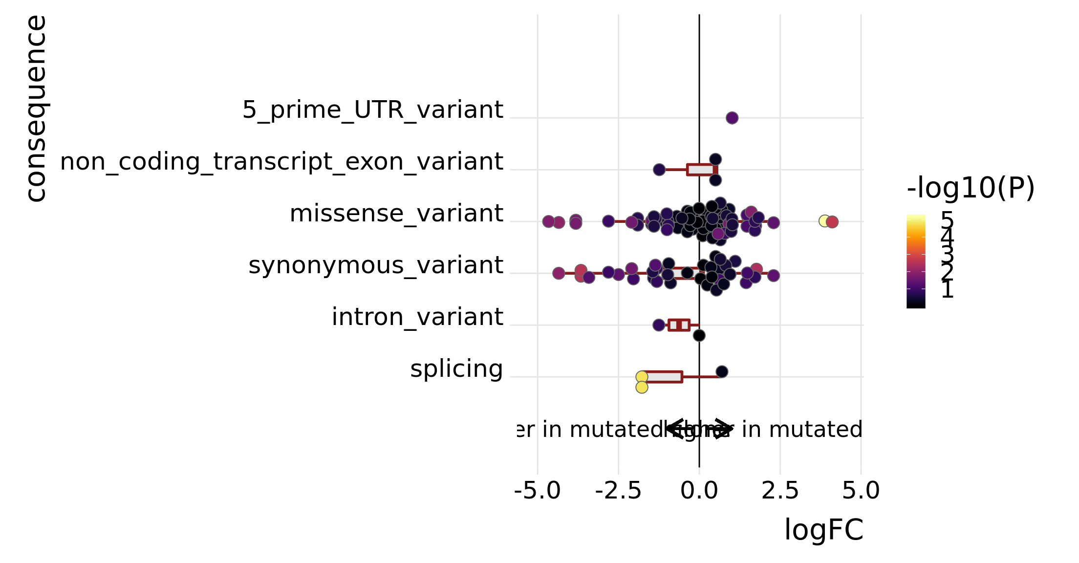
Differential expression transcriptome-wide
First we can look for genes that have any significant difference in expression between clones. The summary below shows the number of significant and non-significant genes at a Benjamini-Hochberg FDR threshold of 10%.
knitr::opts_chunk$set(fig.height = 6, fig.width = 8)
summary(decideTests(de_res$qlf_list$joxm, p.value = 0.1))
assignedclone3-assignedclone2
NotSig 10150
Sig 901 assignedclone3-assignedclone2
NotSig 10502
Sig 549We can view the 10 genes with strongest evidence for differential expression across clones.
Coefficient: assignedclone2 assignedclone3
logFC.assignedclone2 logFC.assignedclone3
ENSG00000205542_TMSB4X -0.2886522 -5.8130458
ENSG00000124508_BTN2A2 -0.2512275 4.1377818
ENSG00000158882_TOMM40L -0.2553535 6.2263232
ENSG00000146776_ATXN7L1 5.8013534 3.3752647
ENSG00000026652_AGPAT4 2.3215386 5.8405432
ENSG00000215271_HOMEZ 4.2232674 2.6794625
ENSG00000175395_ZNF25 -2.1170549 4.6804151
ENSG00000135776_ABCB10 0.6713155 5.0054153
ENSG00000095739_BAMBI 4.5309789 -0.3778691
ENSG00000136158_SPRY2 -1.2049610 4.7778728
logCPM F PValue FDR
ENSG00000205542_TMSB4X 12.468006 91.46976 2.962531e-22 3.273893e-18
ENSG00000124508_BTN2A2 2.498248 47.36794 1.474039e-12 8.144803e-09
ENSG00000158882_TOMM40L 3.337964 38.97201 2.925525e-12 1.077666e-08
ENSG00000146776_ATXN7L1 3.810016 32.87690 2.116125e-11 5.846324e-08
ENSG00000026652_AGPAT4 2.860100 33.06655 5.771600e-11 1.275639e-07
ENSG00000215271_HOMEZ 2.851795 30.02105 1.122804e-10 2.068018e-07
ENSG00000175395_ZNF25 3.174000 29.63095 1.417301e-10 2.237513e-07
ENSG00000135776_ABCB10 2.677297 29.15750 1.989993e-10 2.748926e-07
ENSG00000095739_BAMBI 3.004732 27.60813 6.651894e-10 8.167787e-07
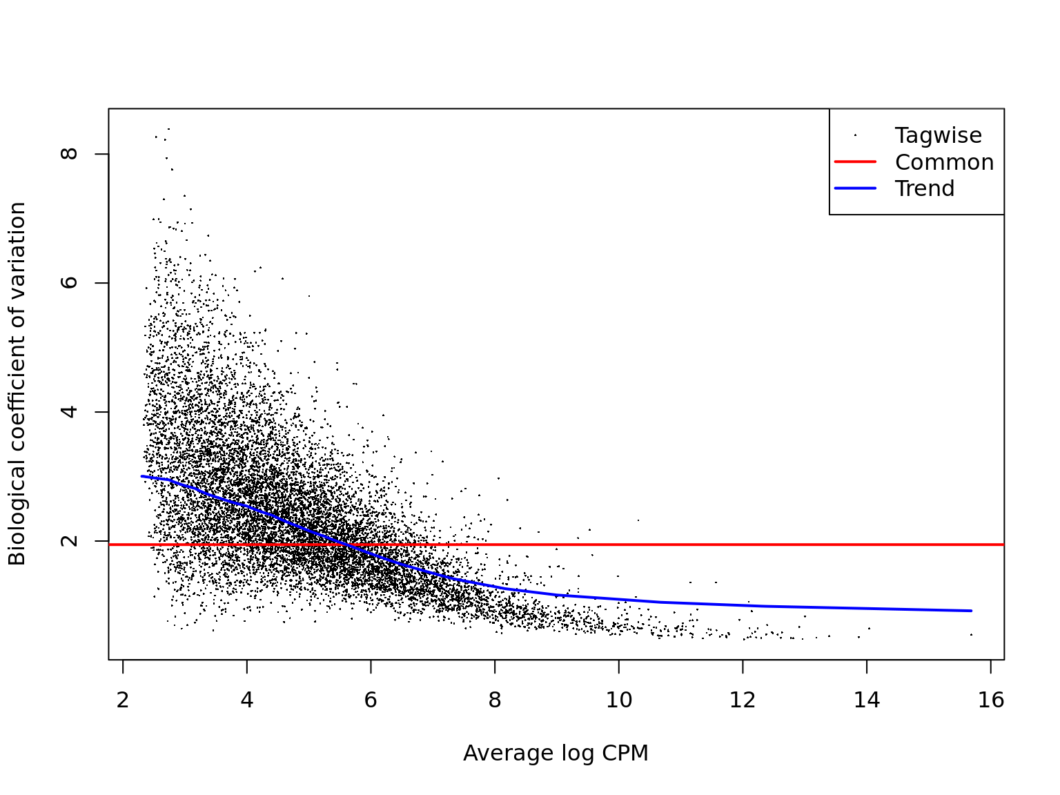
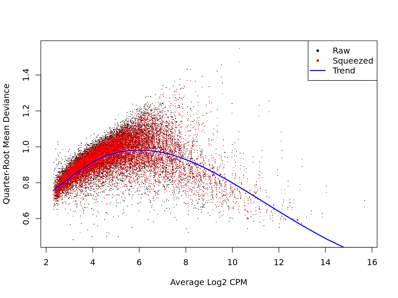
ENSG00000136158_SPRY2 2.677447 37.27297 8.205003e-10 9.067349e-07We can check that the estimates of the biological coefficient of variation from the negative binomial model look sensible. Here they do, so we can expect sensible DE results.
Likewise, a plot of the quasi-likelihood parameter against average gene expression looks smooth and sensible.
Pairwise comparisons of clones
As well as looking for any difference in expression across clones, we can also inspect specific pairwise contrasts of clones for differential expression.
For this donor, we are able to look at 3 pairwise contrasts.
The output below shows the top 10 DE genes for pair of (testable) clones.
cntrsts <- names(de_res$qlf_pairwise$joxm)[-1]
for (i in cntrsts) {
  print(topTags(de_res$qlf_pairwise$joxm[[i]]))
}
Coefficient: assignedclone2
logFC logCPM F PValue
ENSG00000146776_ATXN7L1 5.801353 3.810016 64.75358 3.618933e-12
ENSG00000215271_HOMEZ 4.223267 2.851795 56.91066 3.832169e-11
ENSG00000095739_BAMBI 4.530979 3.004732 46.71443 1.314479e-09
ENSG00000165475_CRYL1 4.020138 3.055068 42.15286 4.773076e-09
ENSG00000256977_LIMS3 3.124759 2.708791 39.15415 2.358976e-08
ENSG00000166896_XRCC6BP1 2.972211 2.628904 35.00854 6.100632e-08
ENSG00000113368_LMNB1 -4.995249 3.932812 34.70055 8.566612e-08
ENSG00000165752_STK32C -5.481150 4.483212 32.82498 1.405996e-07
ENSG00000143845_ETNK2 3.270634 2.816029 33.28608 1.513342e-07
ENSG00000197465_GYPE 3.010858 2.606880 32.67812 1.687145e-07
ensembl_gene_id hgnc_symbol entrezid FDR
ENSG00000146776_ATXN7L1 ENSG00000146776 ATXN7L1 222255 3.999282e-08
ENSG00000215271_HOMEZ ENSG00000215271 HOMEZ 57594 2.117465e-07
ENSG00000095739_BAMBI ENSG00000095739 BAMBI 25805 4.842103e-06
ENSG00000165475_CRYL1 ENSG00000165475 CRYL1 51084 1.318681e-05
ENSG00000256977_LIMS3 ENSG00000256977 LIMS3 96626 5.213808e-05
ENSG00000166896_XRCC6BP1 ENSG00000166896 XRCC6BP1 91419 1.123635e-04
ENSG00000113368_LMNB1 ENSG00000113368 LMNB1 4001 1.352423e-04
ENSG00000165752_STK32C ENSG00000165752 STK32C 282974 1.858215e-04
ENSG00000143845_ETNK2 ENSG00000143845 ETNK2 55224 1.858215e-04
ENSG00000197465_GYPE ENSG00000197465 GYPE 2996 1.864463e-04
Coefficient: assignedclone3
logFC logCPM F PValue
ENSG00000205542_TMSB4X -5.813046 12.468006 182.84733 3.083273e-23
ENSG00000026652_AGPAT4 5.840543 2.860100 65.80971 8.363155e-12
ENSG00000158882_TOMM40L 6.226323 3.337964 60.47867 3.581635e-11
ENSG00000135776_ABCB10 5.005415 2.677297 54.64197 8.190527e-11
ENSG00000124508_BTN2A2 4.137782 2.498248 62.56667 1.483166e-10
ENSG00000129048_ACKR4 8.028290 3.720048 65.44187 3.310506e-10
ENSG00000173295_FAM86B3P 6.964274 3.295641 47.99588 6.618565e-10
ENSG00000180787_ZFP3 5.608020 3.305761 48.06258 1.091002e-09
ENSG00000136158_SPRY2 4.777873 2.677447 45.43698 4.638210e-08
ENSG00000198168_SVIP 5.917955 3.038543 34.42856 7.554858e-08
ensembl_gene_id hgnc_symbol entrezid FDR
ENSG00000205542_TMSB4X ENSG00000205542 TMSB4X 7114 3.407325e-19
ENSG00000026652_AGPAT4 ENSG00000026652 AGPAT4 56895 4.621061e-08
ENSG00000158882_TOMM40L ENSG00000158882 TOMM40L 84134 1.319355e-07
ENSG00000135776_ABCB10 ENSG00000135776 ABCB10 23456 2.262838e-07
ENSG00000124508_BTN2A2 ENSG00000124508 BTN2A2 10385 3.278094e-07
ENSG00000129048_ACKR4 ENSG00000129048 ACKR4 51554 6.097401e-07
ENSG00000173295_FAM86B3P ENSG00000173295 FAM86B3P 286042 1.044882e-06
ENSG00000180787_ZFP3 ENSG00000180787 ZFP3 124961 1.507083e-06
ENSG00000136158_SPRY2 ENSG00000136158 SPRY2 10253 5.695206e-05
ENSG00000198168_SVIP ENSG00000198168 SVIP 258010 7.523350e-05
Coefficient: -1*assignedclone2 1*assignedclone3
logFC logCPM F PValue
ENSG00000205542_TMSB4X -5.524394 12.468006 167.09909 4.400831e-22
ENSG00000175395_ZNF25 6.797470 3.174000 53.10092 1.265384e-10
ENSG00000124508_BTN2A2 4.389009 2.498248 54.14334 1.147322e-09
ENSG00000136158_SPRY2 5.982834 2.677447 60.81381 1.644934e-09
ENSG00000158882_TOMM40L 6.481677 3.337964 43.32876 6.013150e-09
ENSG00000039139_DNAH5 5.420749 3.262779 41.04082 9.408878e-09
ENSG00000100084_HIRA 5.722823 3.119595 43.45990 1.977958e-08
ENSG00000164099_PRSS12 5.677707 3.222941 36.68476 3.308745e-08
ENSG00000148840_PPRC1 5.234448 2.909858 34.39080 1.243506e-07
ENSG00000165752_STK32C 7.004519 4.483212 32.86562 1.384803e-07
ensembl_gene_id hgnc_symbol entrezid FDR
ENSG00000205542_TMSB4X ENSG00000205542 TMSB4X 7114 4.863358e-18
ENSG00000175395_ZNF25 ENSG00000175395 ZNF25 219749 6.991878e-07
ENSG00000124508_BTN2A2 ENSG00000124508 BTN2A2 10385 4.226351e-06
ENSG00000136158_SPRY2 ENSG00000136158 SPRY2 10253 4.544540e-06
ENSG00000158882_TOMM40L ENSG00000158882 TOMM40L 84134 1.329026e-05
ENSG00000039139_DNAH5 ENSG00000039139 DNAH5 1767 1.732958e-05
ENSG00000100084_HIRA ENSG00000100084 HIRA 7290 3.122630e-05
ENSG00000164099_PRSS12 ENSG00000164099 PRSS12 8492 4.570617e-05
ENSG00000148840_PPRC1 ENSG00000148840 PPRC1 23082 1.526887e-04
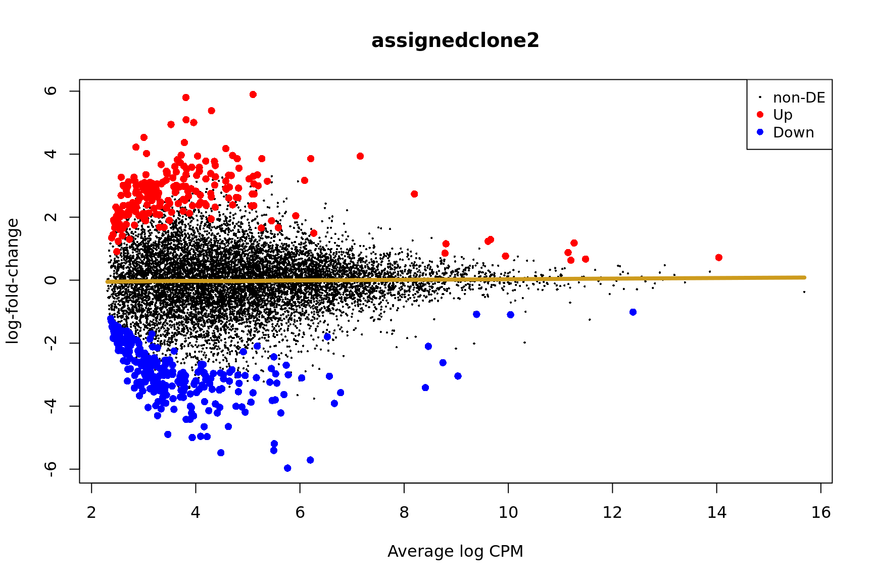
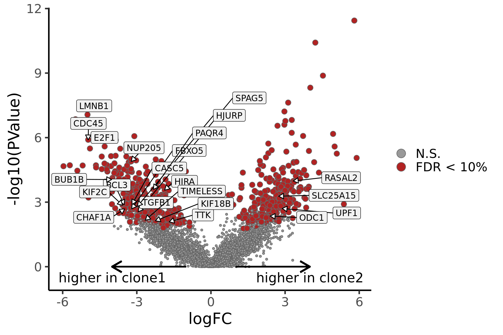
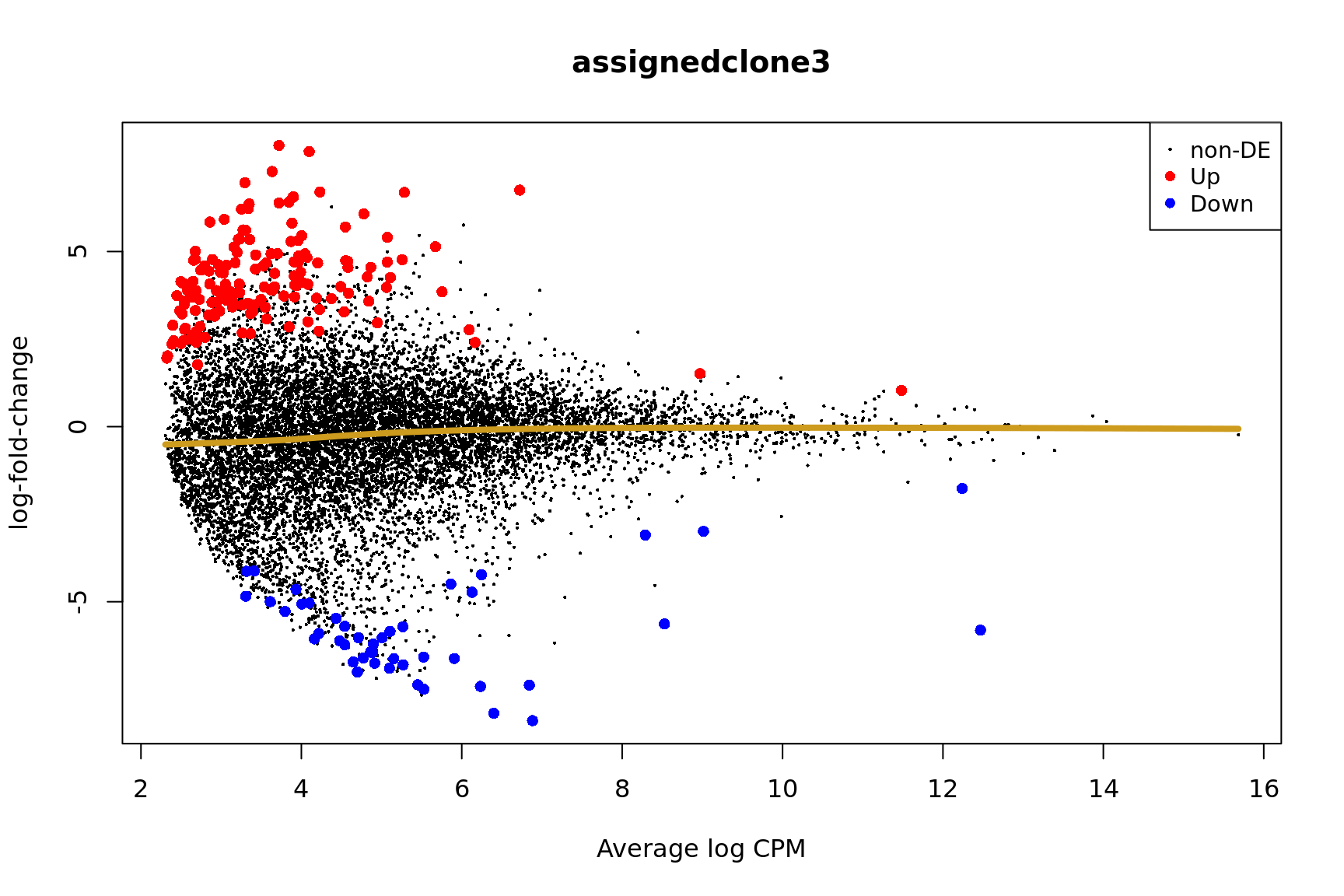
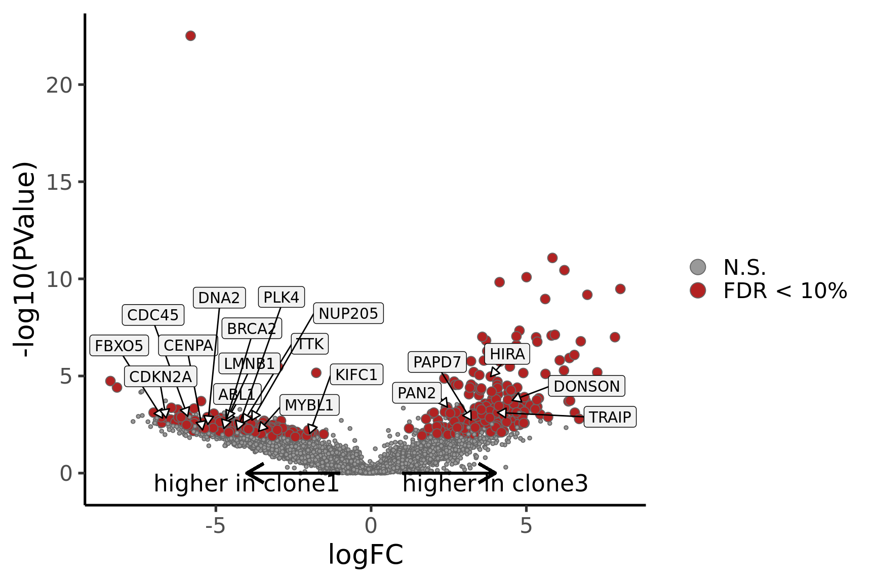
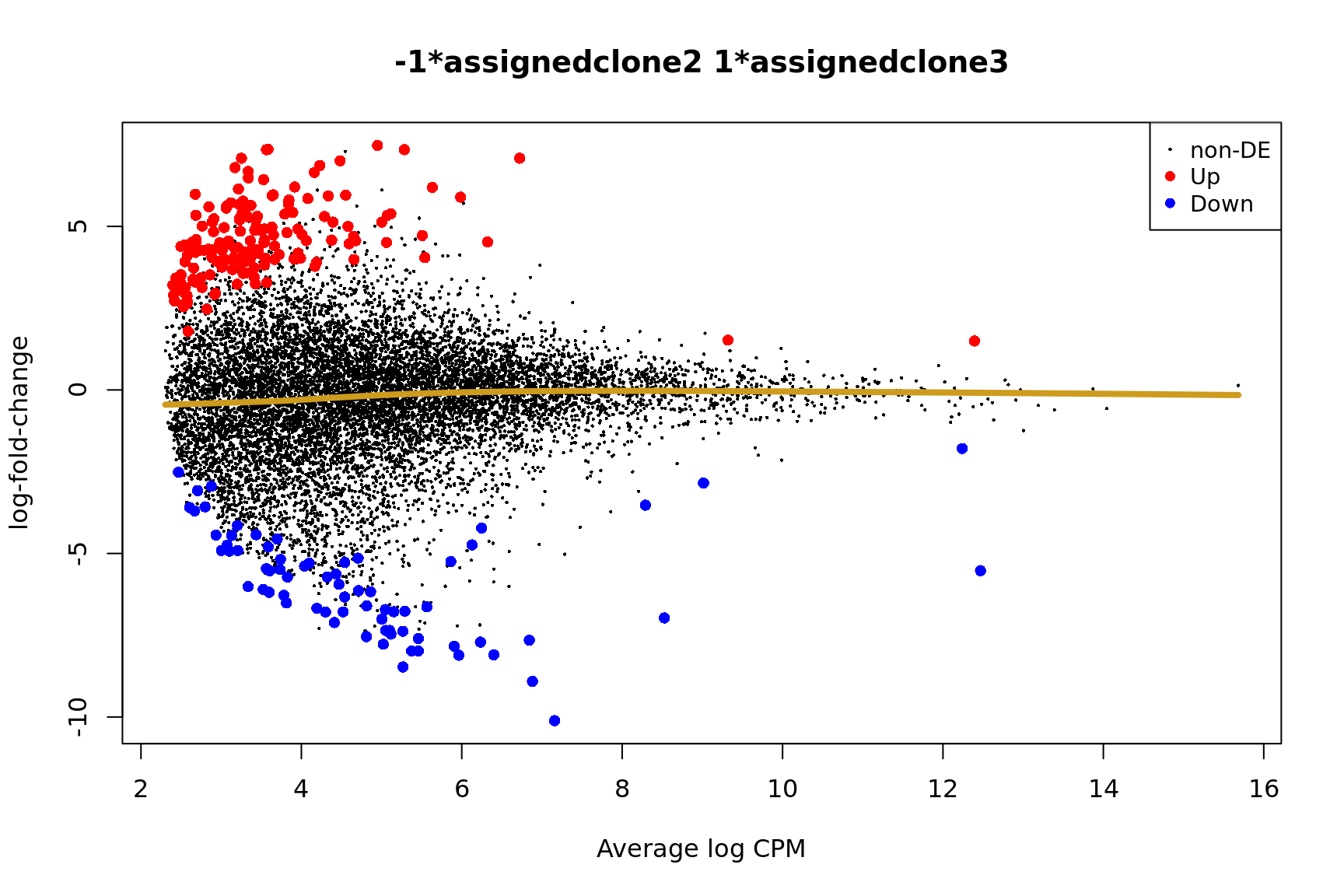
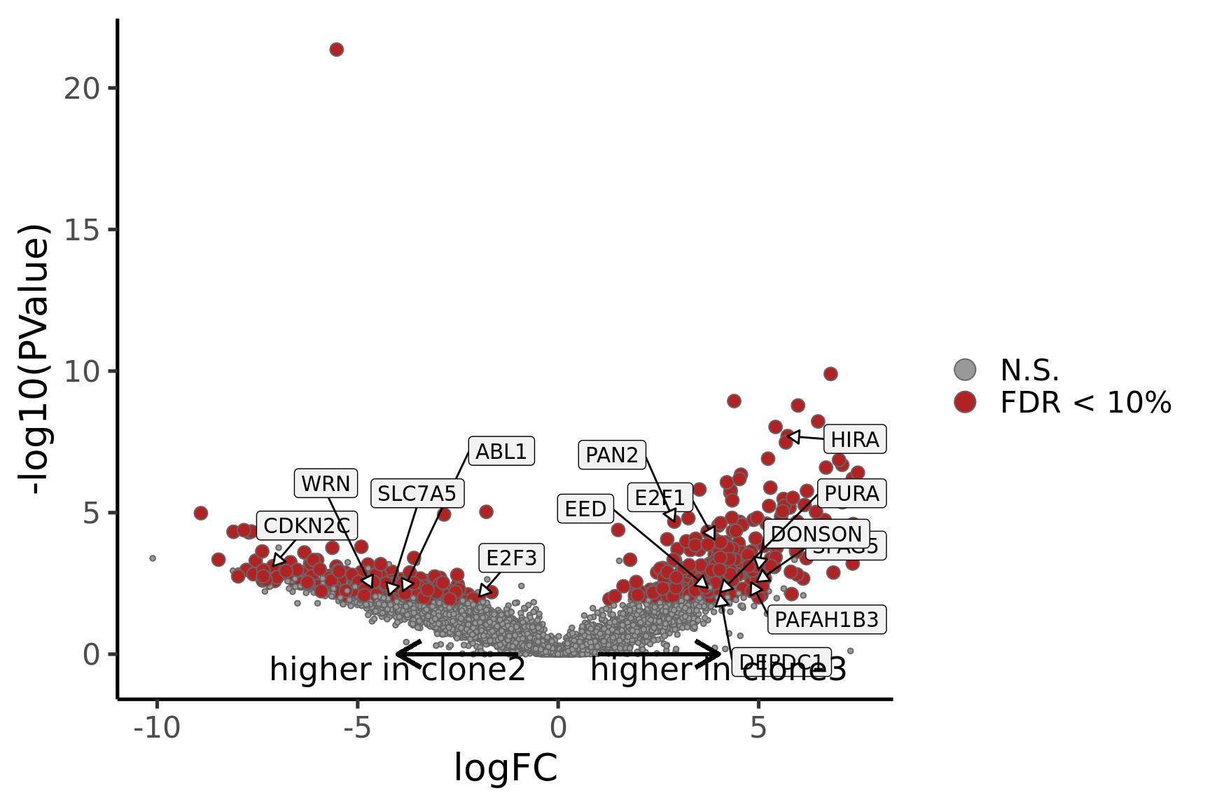
ENSG00000165752_STK32C ENSG00000165752 STK32C 282974 1.530346e-04Below we see the following plots for each pairwise comparison:
- A “mean-difference” plot: log-fold-change (between clones) vs average expression;
- A “volcano plot”: -log10(PValue) vs log-fold-change between clones.
In the MD plots we see logFC distributions centred around zero as we would hope (gold line in plots shows lowess curve through points).
for (i in cntrsts) {
  plotMD(de_res$qlf_pairwise$joxm[[i]], p.value = 0.1)
  lines(lowess(x = de_res$qlf_pairwise$joxm[[i]]$table$logCPM,
               y = de_res$qlf_pairwise$joxm[[i]]$table$logFC),
        col = "goldenrod3", lwd = 4)

  de_tab <- de_res$qlf_pairwise$joxm[[i]]$table
  de_tab[["gene"]] <- rownames(de_tab)
  de_tab <- de_tab %>%
    dplyr::mutate(FDR = adj_pvalues(ihw(PValue ~ logCPM, alpha = 0.1)),
                  sig = FDR < 0.1,
                  signed_F = sign(logFC) * F)
  de_tab[["lab"]] <- ""
  int_genes_entrezid <- c(Hs.H$HALLMARK_G2M_CHECKPOINT, Hs.H$HALLMARK_E2F_TARGETS,
                          Hs.c2$ROSTY_CERVICAL_CANCER_PROLIFERATION_CLUSTER)
  mm <- match(int_genes_entrezid, de_tab$entrezid)
  mm <- mm[!is.na(mm)]
  int_genes_hgnc <- de_tab$hgnc_symbol[mm]
  int_genes_hgnc <- c(int_genes_hgnc, "MYBL1")
  genes_to_label <- (de_tab[["hgnc_symbol"]] %in% int_genes_hgnc &
                       de_tab[["FDR"]] < 0.1)
  de_tab[["lab"]][genes_to_label] <-
    de_tab[["hgnc_symbol"]][genes_to_label]

  p_vulcan <- ggplot(de_tab, aes(x = logFC, y = -log10(PValue), fill = sig,
                     label = lab)) +
    geom_point(aes(size = sig), pch = 21, colour = "gray40") +
    geom_label_repel(show.legend = FALSE,
                     arrow = arrow(type = "closed", length = unit(0.25, "cm")),
                     nudge_x = 0.2, nudge_y = 0.3, fill = "gray95") +
    geom_segment(aes(x = -1, y = 0, xend = -4, yend = 0),
                 colour = "black", size = 1, arrow = arrow(length = unit(0.5, "cm"))) +
    annotate("text", x = -4, y = -0.5, size = 6,
             label = paste("higher in", strsplit(i, "_")[[1]][2])) +
    geom_segment(aes(x = 1, y = 0, xend = 4, yend = 0),
                 colour = "black", size = 1, arrow = arrow(length = unit(0.5, "cm"))) +
    annotate("text", x = 4, y = -0.5, size = 6,
             label = paste("higher in", strsplit(i, "_")[[1]][1])) +
    scale_fill_manual(values = c("gray60", "firebrick"),
                      label = c("N.S.", "FDR < 10%"), name = "") +
    scale_size_manual(values = c(1, 3), guide = FALSE) +
    guides(alpha = FALSE,
           fill = guide_legend(override.aes = list(size = 5))) +
    theme_classic(20) + theme(legend.position = "right")
  print(p_vulcan)

  ggsave(paste0("figures/donor_specific/carderelax_joxm_volcano_", i, ".png"),
         plot = p_vulcan, height = 6, width = 9)
  ggsave(paste0("figures/donor_specific/carderelax_joxm_volcano_", i, ".pdf"),
         plot = p_vulcan, height = 6, width = 9)
  ggsave(paste0("figures/donor_specific/carderelax_joxm_volcano_", i, ".svg"),
         plot = p_vulcan, height = 6, width = 9)
}
Gene set enrichment results
We extend our analysis from looking at differential expression for single genes to looking for enrichment in gene sets. We use gene sets from the MSigDB collection.
We use the camera method from the limma package to conduct competitive gene set testing. This method uses the full distributions of logFC statistics from pairwise clone contrasts to identify significantly enriched gene sets.
MSigDB Hallmark gene sets
We look primarily at the “Hallmark” collection of gene sets from MSigDB.
for (i in cntrsts) {
print(i)
cam_H_pw <- de_res$camera$H$joxm[[i]]$logFC
cam_H_pw[["geneset"]] <- rownames(de_res$camera$H$joxm[[i]]$logFC)
cam_H_pw <- cam_H_pw %>%
dplyr::mutate(sig = FDR < 0.05)
print(head(cam_H_pw))
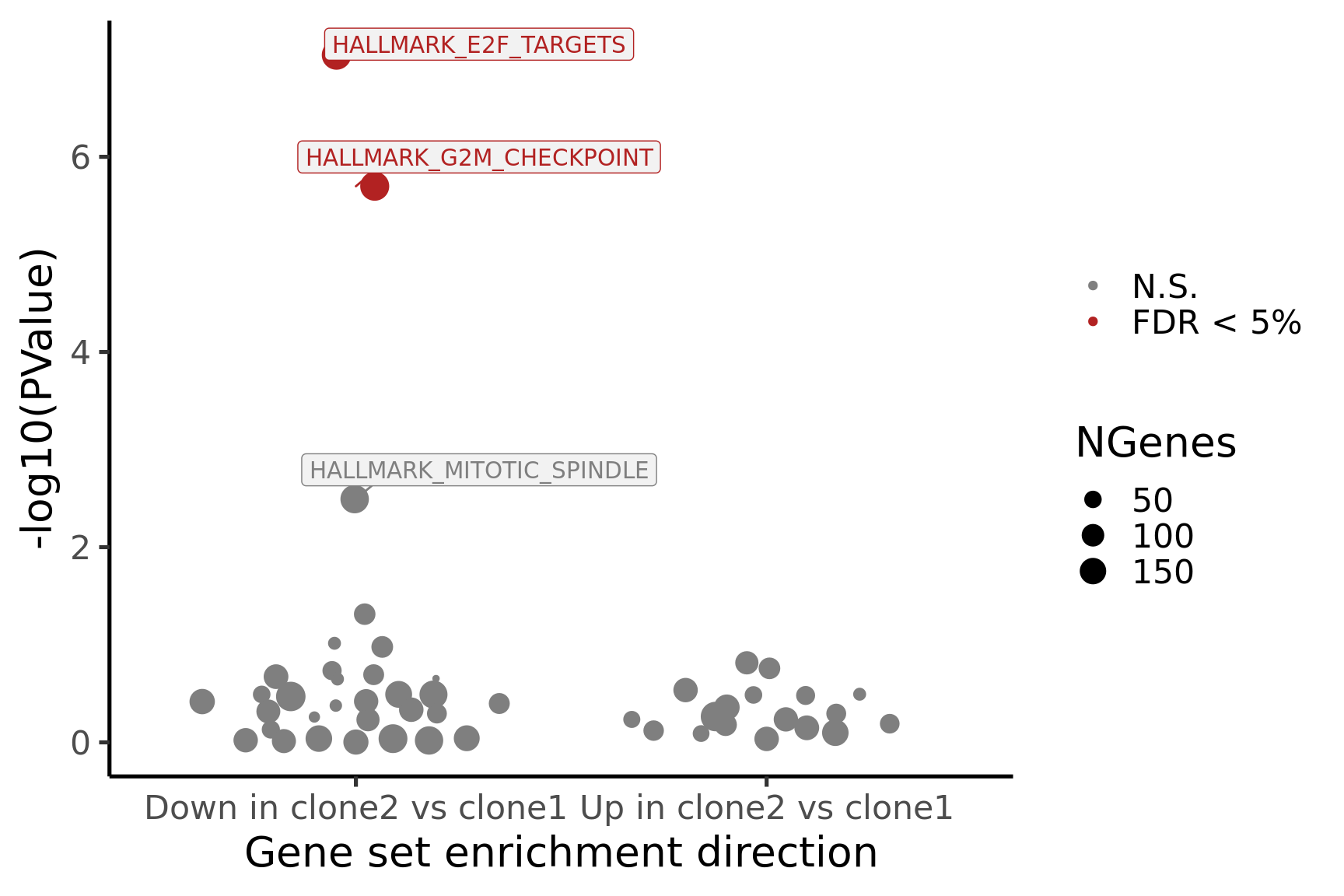
}[1] "clone2_clone1"
NGenes Direction PValue FDR
1 197 Down 9.059034e-08 4.529517e-06
2 190 Down 2.002810e-06 5.007025e-05
3 181 Down 3.216112e-03 5.360186e-02
4 88 Down 4.855505e-02 6.069381e-01
5 23 Down 9.654137e-02 8.064825e-01
6 90 Down 1.052216e-01 8.064825e-01
geneset sig
1 HALLMARK_E2F_TARGETS TRUE
2 HALLMARK_G2M_CHECKPOINT TRUE
3 HALLMARK_MITOTIC_SPINDLE FALSE
4 HALLMARK_ALLOGRAFT_REJECTION FALSE
5 HALLMARK_WNT_BETA_CATENIN_SIGNALING FALSE
6 HALLMARK_INFLAMMATORY_RESPONSE FALSE
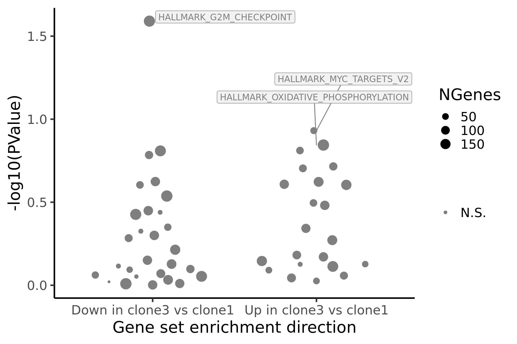
[1] "clone3_clone1"
NGenes Direction PValue FDR geneset
1 190 Down 0.02567449 0.9567097 HALLMARK_G2M_CHECKPOINT
2 56 Up 0.11722963 0.9567097 HALLMARK_MYC_TARGETS_V2
3 198 Up 0.14312855 0.9567097 HALLMARK_OXIDATIVE_PHOSPHORYLATION
4 71 Up 0.15442973 0.9567097 HALLMARK_COAGULATION
5 181 Down 0.15515689 0.9567097 HALLMARK_MITOTIC_SPINDLE
6 88 Down 0.16432866 0.9567097 HALLMARK_ALLOGRAFT_REJECTION
sig
1 FALSE
2 FALSE
3 FALSE
4 FALSE
5 FALSE
6 FALSE
[1] "clone3_clone2"
NGenes Direction PValue FDR geneset
1 197 Up 0.03522298 0.9512593 HALLMARK_E2F_TARGETS
2 56 Up 0.08925877 0.9512593 HALLMARK_MYC_TARGETS_V2
3 156 Up 0.09149777 0.9512593 HALLMARK_GLYCOLYSIS
4 123 Up 0.17229713 0.9512593 HALLMARK_IL2_STAT5_SIGNALING
5 123 Down 0.23334204 0.9512593 HALLMARK_INTERFERON_GAMMA_RESPONSE
6 116 Up 0.25855405 0.9512593 HALLMARK_MYOGENESIS
sig
1 FALSE
2 FALSE
3 FALSE
4 FALSE
5 FALSE
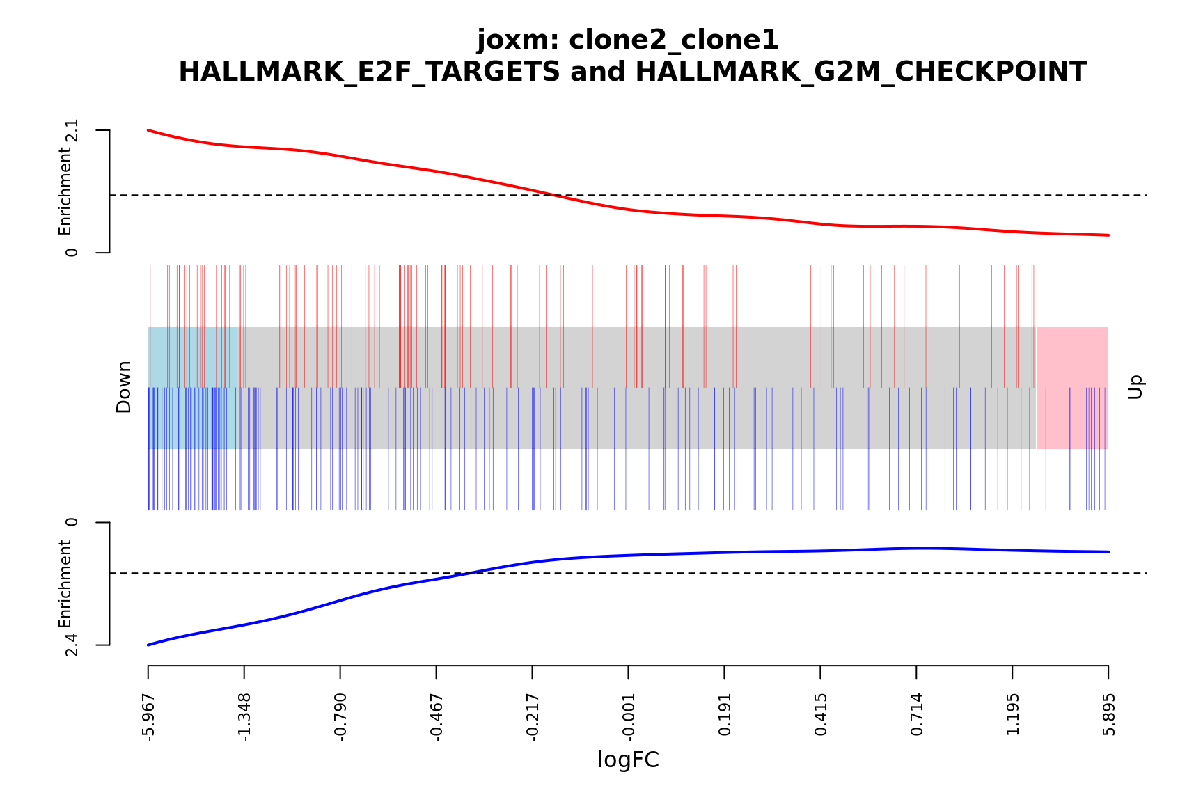
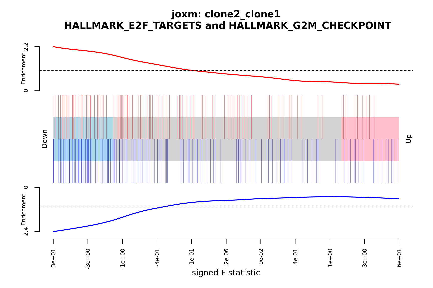
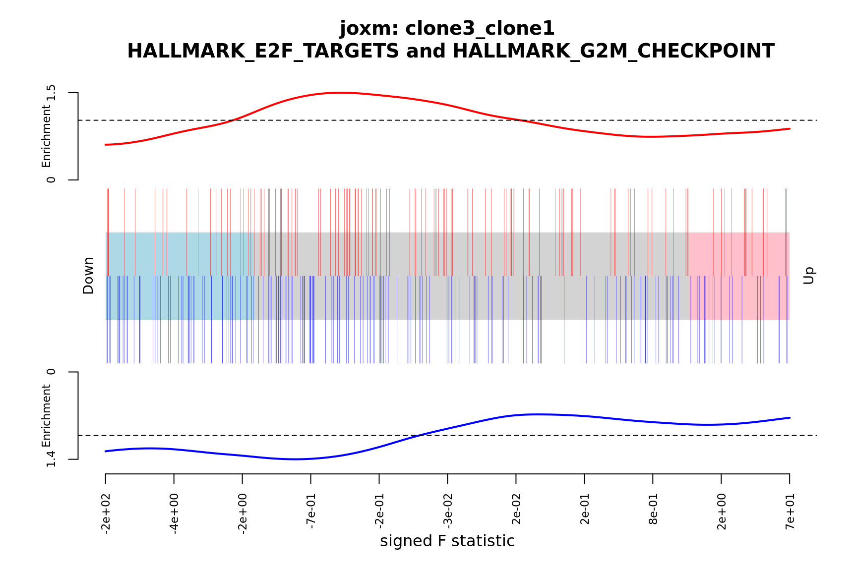
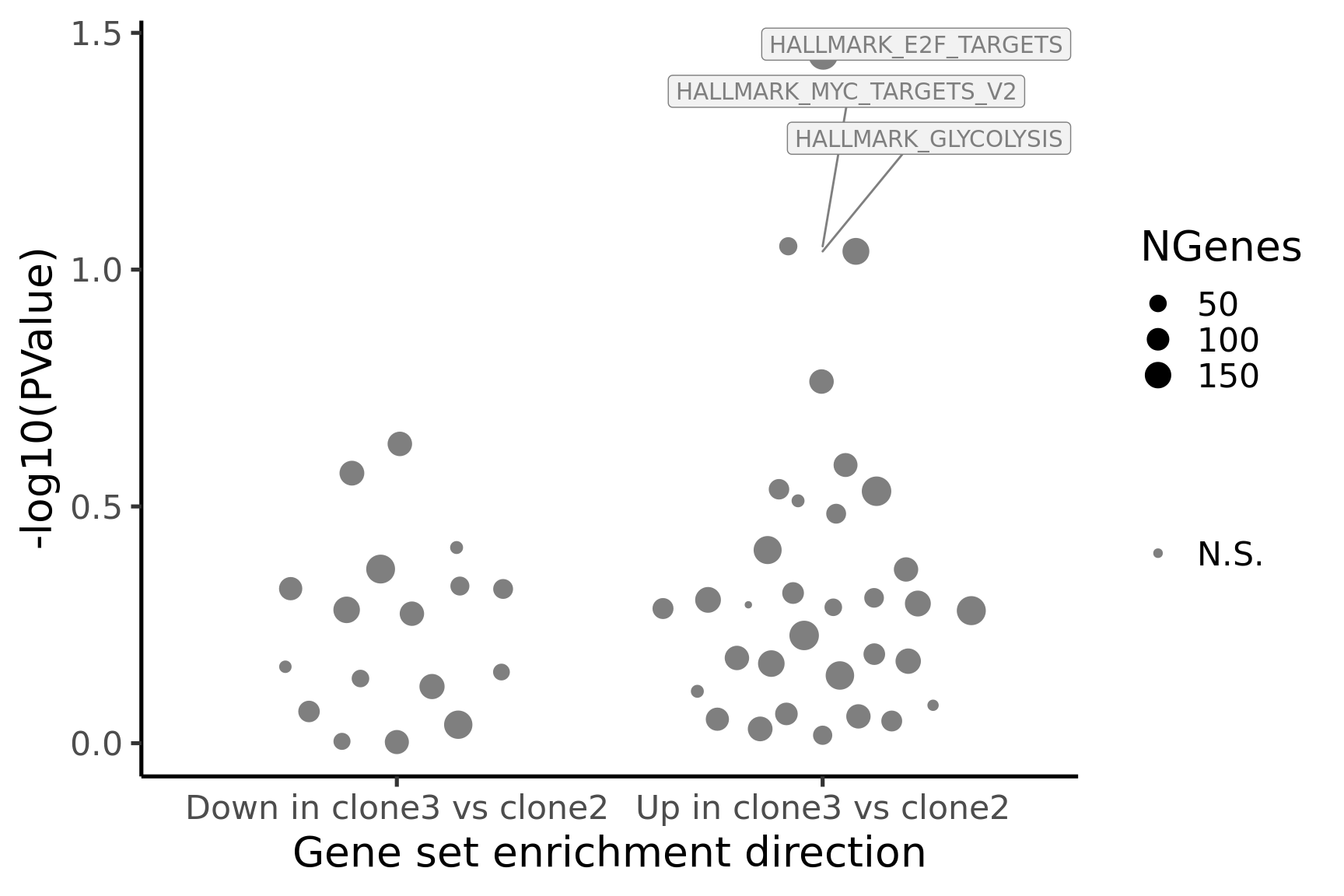
6 FALSEBelow we see the following plots for each pairwise comparison:
- A -log10(PValue) vs direction plot for enrichment of each of the 50 Hallmark gene sets;
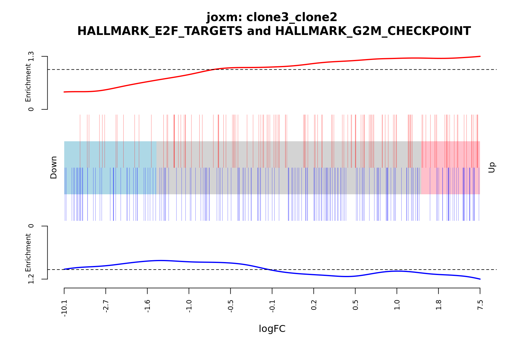
- A logFC “barcode plot”: distribution of the logFC statistics for genes in the E2F targets and G2M checkpoint gene sets relative to all other genes;
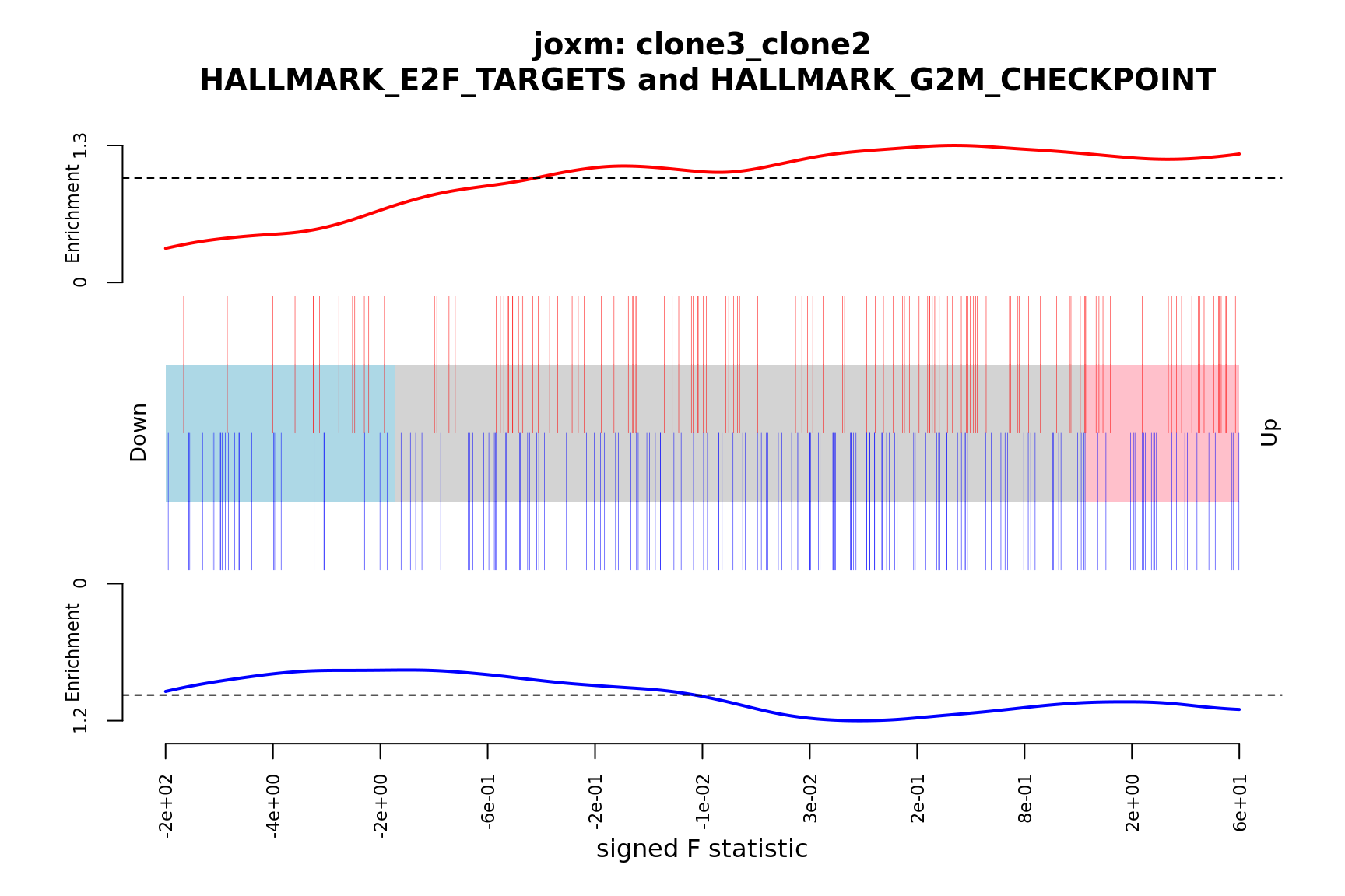
- A signed-F “barcode plot”: distribution of the signed F statistics for genes in the E2F targets and G2M checkpoint gene sets relative to all other genes.
for (i in cntrsts) {
  cam_H_pw <- de_res$camera$H$joxm[[i]]$logFC
  cam_H_pw[["geneset"]] <- rownames(de_res$camera$H$joxm[[i]]$logFC)
  cam_H_pw <- cam_H_pw %>%
    dplyr::mutate(sig = FDR < 0.05)
  cam_H_pw[["lab"]] <- ""
  cam_H_pw[["lab"]][1:3] <-
    cam_H_pw[["geneset"]][1:3]
  cam_H_pw[["Direction"]][cam_H_pw[["Direction"]] == "Up"] <-
    paste("Up in", strsplit(i, "_")[[1]][1], "vs", strsplit(i, "_")[[1]][2])
  cam_H_pw[["Direction"]][cam_H_pw[["Direction"]] == "Down"] <-
    paste("Down in", strsplit(i, "_")[[1]][1], "vs", strsplit(i, "_")[[1]][2])
  de_tab <- de_res$qlf_pairwise$joxm[[i]]$table
  de_tab[["gene"]] <- rownames(de_tab)
  de_tab <- de_tab %>%
    dplyr::mutate(FDR = adj_pvalues(ihw(PValue ~ logCPM, alpha = 0.1)),
                  sig = FDR < 0.1,
                  signed_F = sign(logFC) * F)

  p_hallmark <- cam_H_pw %>%
    ggplot(aes(x = Direction, y = -log10(PValue), colour = sig,
               label = lab)) +
    ggbeeswarm::geom_quasirandom(aes(size = NGenes)) +
    geom_label_repel(show.legend = FALSE,
                     nudge_y = 0.3, nudge_x = 0.3, fill = "gray95") +
    scale_colour_manual(values = c("gray50", "firebrick"),
                        label = c("N.S.", "FDR < 5%"), name = "") +
    guides(alpha = FALSE,
           fill = guide_legend(override.aes = list(size = 5))) +
    xlab("Gene set enrichment direction") +
    theme_classic(20) + theme(legend.position = "right")
  print(p_hallmark)

  ggsave(paste0("figures/donor_specific/carderelax_joxm_camera_H_", i, ".png"),
         plot = p_hallmark, height = 6, width = 9)
  ggsave(paste0("figures/donor_specific/carderelax_joxm_camera_H_", i, ".png"),
         plot = p_hallmark, height = 6, width = 9)
  ggsave(paste0("figures/donor_specific/carderelax_joxm_camera_H_", i, ".png"),
         plot = p_hallmark, height = 6, width = 9)

  idx <- ids2indices(Hs.H, id = de_tab$entrezid)
  barcodeplot(de_tab$logFC, index = idx$HALLMARK_E2F_TARGETS,
              index2 = idx$HALLMARK_G2M_CHECKPOINT, xlab = "logFC",
              main = paste0("joxm: ", i, "\n HALLMARK_E2F_TARGETS and HALLMARK_G2M_CHECKPOINT"))

  png(paste0("figures/donor_specific/carderelax_joxm_camera_H_", i, "_barcode_logFC_E2F_G2M.png"),
      height = 400, width = 600)
  barcodeplot(de_tab$logFC, index = idx$HALLMARK_E2F_TARGETS,
              index2 = idx$HALLMARK_G2M_CHECKPOINT, xlab = "logFC",
              main = paste0("joxm: ", i, "\n HALLMARK_E2F_TARGETS and HALLMARK_G2M_CHECKPOINT"))
  dev.off()

  barcodeplot(de_tab$signed_F, index = idx$HALLMARK_E2F_TARGETS,
              index2 = idx$HALLMARK_G2M_CHECKPOINT, xlab = "signed F statistic",
              main = paste0("joxm: ", i, "\n HALLMARK_E2F_TARGETS and HALLMARK_G2M_CHECKPOINT"))
  png(paste0("figures/donor_specific/carderelax_joxm_camera_H_", i, "_barcode_signedF_E2F_G2M.png"),
      height = 400, width = 600)
  barcodeplot(de_tab$signed_F, index = idx$HALLMARK_E2F_TARGETS,
              index2 = idx$HALLMARK_G2M_CHECKPOINT, xlab = "signed F statistic",
              main = paste0("joxm: ", i, "\n HALLMARK_E2F_TARGETS and HALLMARK_G2M_CHECKPOINT"))
  dev.off()
} 

One could carry out similar analyses and produce similar plots for the c2 and c6 MSigDB gene set collections.
Test for difference in cell cycle phases by clone
We observe differing proportions of cells in different phases of the cell cycle by clone.
as.data.frame(colData(de_res[["sce_list_unst"]][["joxm"]])) %>%
    dplyr::mutate(Cell_Cycle = factor(cyclone_phase, levels = c("G2M", "S", "G1")),
                  assigned = factor(assigned, levels = c("clone3", "clone2", "clone1"))) %>%
  ggplot(aes(x = assigned, fill = Cell_Cycle)) +
  geom_bar() +
  scale_fill_manual(values = c("#ff6a5c", "#ccdfcb", "#414141")) +
  coord_flip() +
  guides(fill = guide_legend(reverse = TRUE)) +
  theme(axis.title.y = element_blank())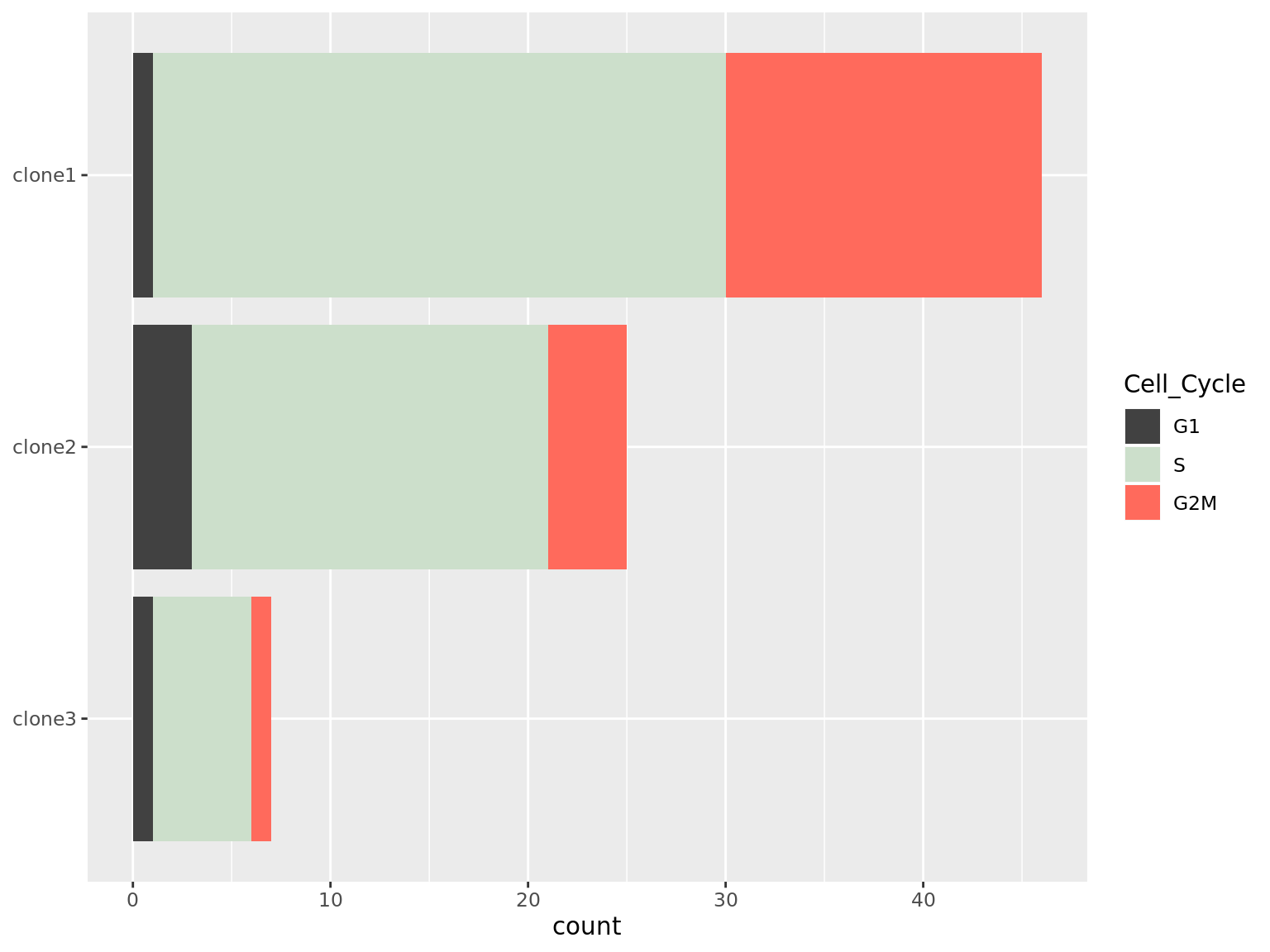
as.data.frame(colData(de_res[["sce_list_unst"]][["joxm"]])) %>%
    dplyr::mutate(Cell_Cycle = factor(cyclone_phase, levels = c("G2M", "S", "G1")),
                  assigned = factor(assigned, levels = c("clone3", "clone2", "clone1"))) %>%
  ggplot(aes(x = assigned, fill = Cell_Cycle)) +
  geom_bar(position = "fill") +
  scale_fill_manual(values = c("#ff6a5c", "#ccdfcb", "#414141")) +
  coord_flip() +
  ylab("proportion") +
  guides(fill = guide_legend(reverse = TRUE)) +
  theme(axis.title.y = element_blank())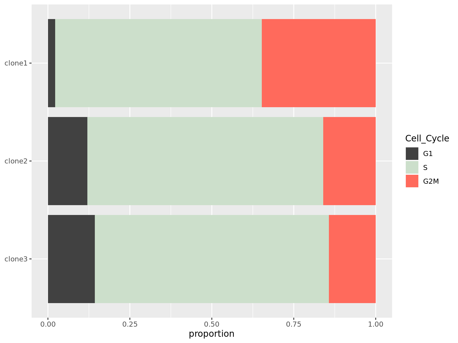
A Fisher Exact Test can provide some guidance about whether or not these differences in cell cycle proportions are expected by chance.
freqs <- as.matrix(table(
    de_res[["sce_list_unst"]][["joxm"]]$assigned,
    de_res[["sce_list_unst"]][["joxm"]]$cyclone_phase))
fisher.test(freqs)
    Fisher's Exact Test for Count Data

data:  freqs
p-value = 0.1335
alternative hypothesis: two.sided
We can also test just for differences in proportions between clone1 and clone2.
    Fisher's Exact Test for Count Data

data:  freqs[-3, ]
p-value = 0.07296
alternative hypothesis: two.sided
PCA plots
Principal component analysis can reveal global structure from single-cell transcriptomic profiles.
choose_joxm_cells <- (sce_joxm$well_condition == "unstimulated" &
                          sce_joxm$assigned != "unassigned")
pca_unst <- reducedDim(runPCA(sce_joxm[, choose_joxm_cells],
                              ntop = 500, ncomponents = 10), "PCA")
pca_unst <- data.frame(
    PC1 = pca_unst[, 1], PC2 = pca_unst[, 2],
    PC3 = pca_unst[, 3], PC4 = pca_unst[, 4],
    PC5 = pca_unst[, 5], PC6 = pca_unst[, 6],
    clone = sce_joxm[, choose_joxm_cells]$assigned,
    nvars_cloneid = sce_joxm[, choose_joxm_cells]$nvars_cloneid,
    cyclone_phase = sce_joxm[, choose_joxm_cells]$cyclone_phase,
    G1 = sce_joxm[, choose_joxm_cells]$G1,
    G2M = sce_joxm[, choose_joxm_cells]$G2M,
    S = sce_joxm[, choose_joxm_cells]$S,
    clone1_prob = sce_joxm[, choose_joxm_cells]$clone1_prob,
    clone2_prob = sce_joxm[, choose_joxm_cells]$clone2_prob,
    clone3_prob = sce_joxm[, choose_joxm_cells]$clone3_prob,
    RPS6KA2 = as.vector(logcounts(sce_joxm[grep("RPS6KA2", rownames(sce_joxm)), choose_joxm_cells]))
    )

ggplot(pca_unst, aes(x = PC1, y = PC2, fill = clone)) +
    geom_point(pch = 21, size = 4, colour = "gray30") +
    scale_fill_brewer(palette = "Accent", name = "assigned\nclone") +
    theme_classic(14)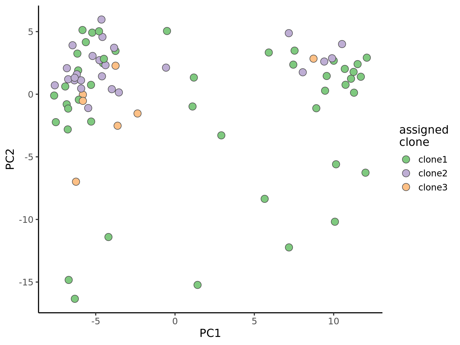
ggplot(pca_unst, aes(x = PC2, y = PC3, fill = clone)) +
    geom_point(pch = 21, size = 4, colour = "gray30") +
    scale_fill_brewer(palette = "Accent", name = "assigned\nclone") +
    theme_classic(14)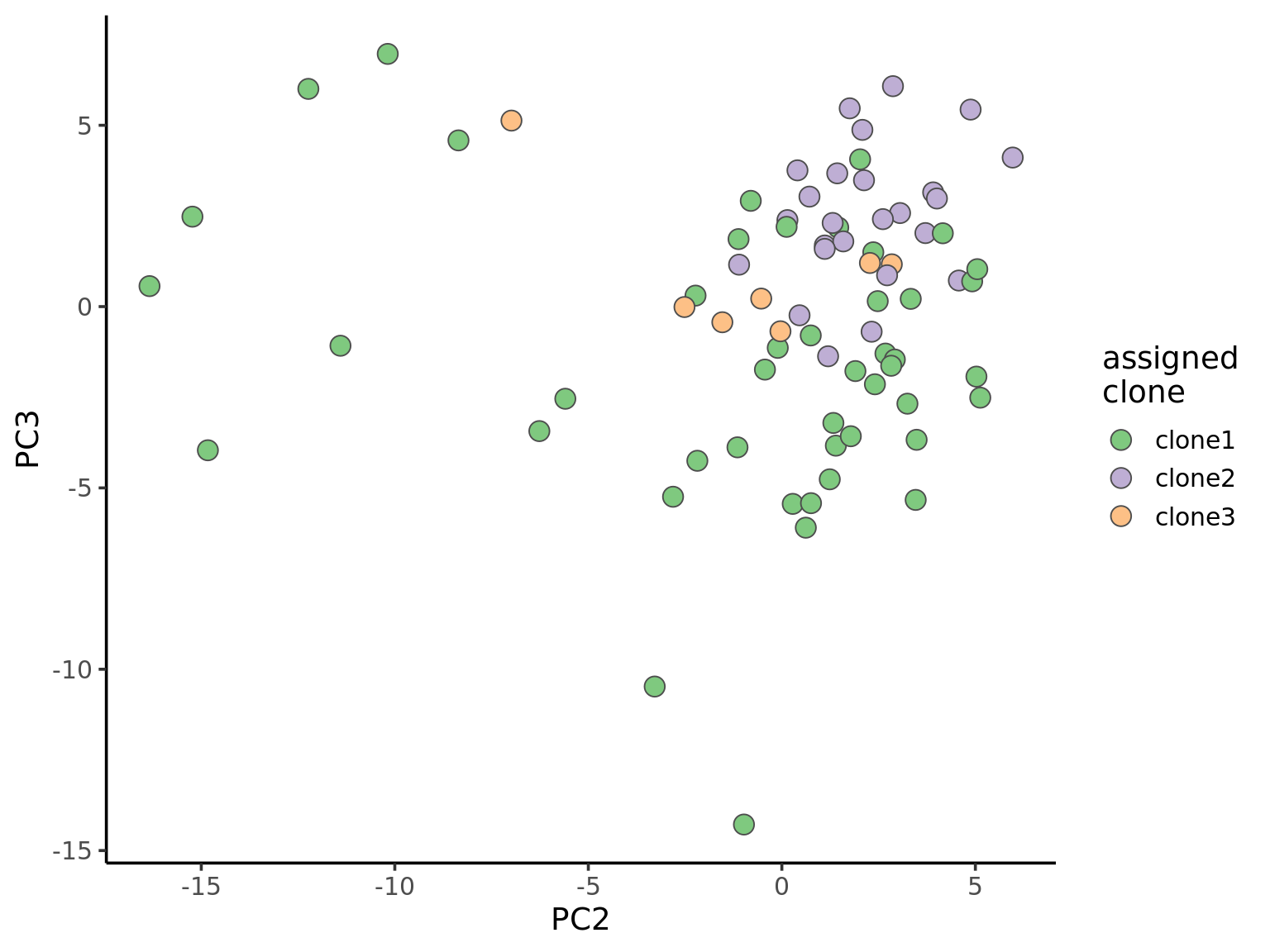
ggplot(pca_unst, aes(x = PC2, y = PC4, fill = clone)) +
    geom_point(pch = 21, size = 4, colour = "gray30") +
    scale_fill_brewer(palette = "Accent", name = "assigned\nclone") +
    theme_classic(14)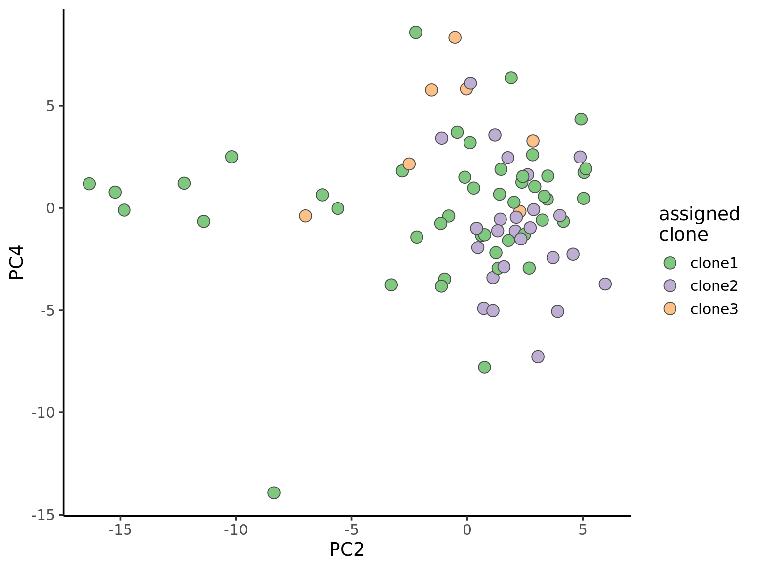
ggplot(pca_unst, aes(x = PC3, y = PC4, fill = clone)) +
    geom_point(pch = 21, size = 4, colour = "gray30") +
    scale_fill_brewer(palette = "Accent", name = "assigned\nclone") +
    theme_classic(14)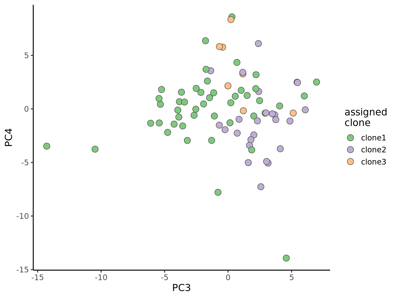
Let us also look at PCA with cells coloured by the posterior probability of assignment to the various clones.
ppc1 <- ggplot(pca_unst, aes(x = PC1, y = PC2, fill = clone1_prob)) +
  geom_point(pch = 21, size = 4, colour = "gray30") +
  scale_fill_viridis(option = "A", name = "clone1\nposterior\nprobability") +
  theme_classic(14)

ppc2 <- ggplot(pca_unst, aes(x = PC1, y = PC2, fill = clone2_prob)) +
  geom_point(pch = 21, size = 4, colour = "gray30") +
  scale_fill_viridis(option = "A", name = "clone2\nposterior\nprobability") +
  theme_classic(14)

ppc3 <- ggplot(pca_unst, aes(x = PC1, y = PC2, fill = clone3_prob)) +
  geom_point(pch = 21, size = 4, colour = "gray30") +
  scale_fill_viridis(option = "A", name = "clone3\nposterior\nprobability") +
  theme_classic(14)

plot_grid(ppc1, ppc2, ppc3, labels = "auto", ncol = 1)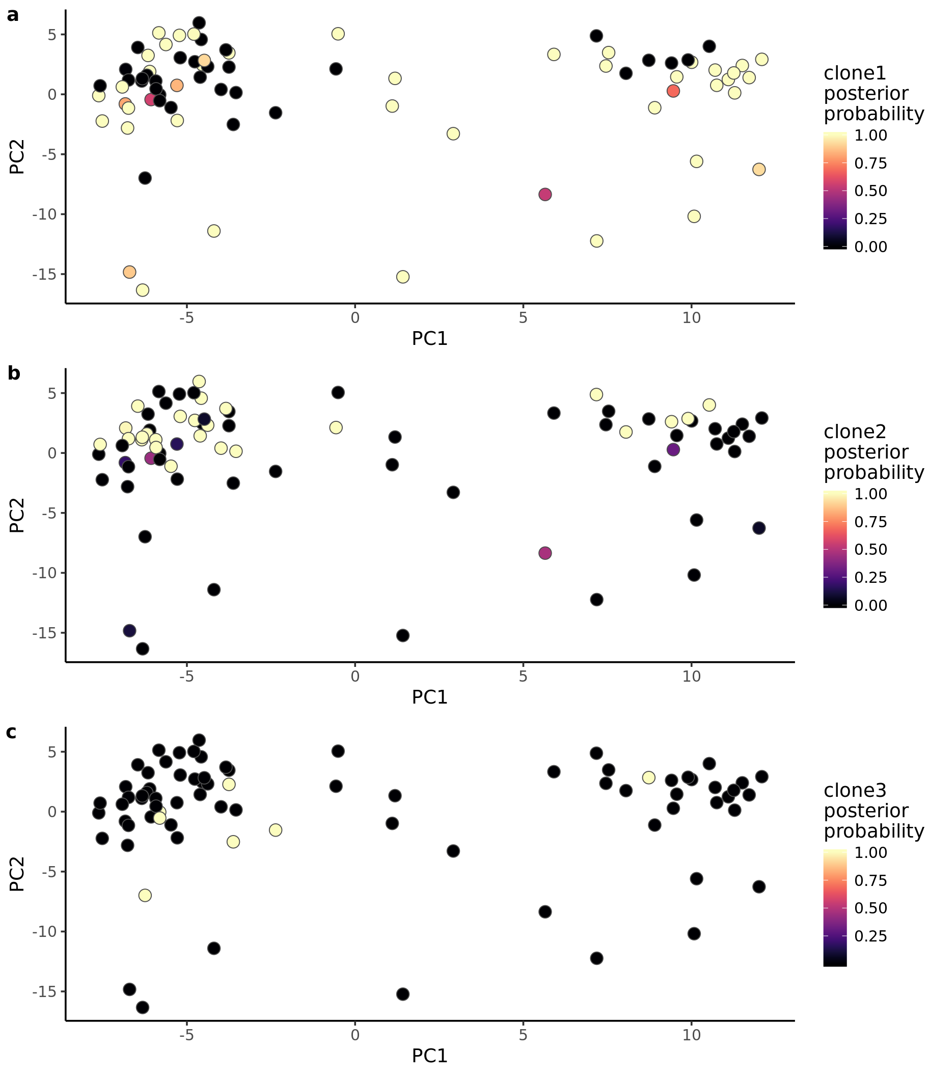
ggsave("figures/donor_specific/carderelax_joxm_pca_pc1_pc2_clone_probs.png", height = 11, width = 9.5)
ggsave("figures/donor_specific/carderelax_joxm_pca_pc1_pc2_clone_probs.pdf", height = 11, width = 9.5)
ggsave("figures/donor_specific/carderelax_joxm_pca_pc1_pc2_clone_probs.svg", height = 11, width = 9.5)

ppc1 <- ggplot(pca_unst, aes(x = PC2, y = PC3, fill = clone1_prob)) +
  geom_point(pch = 21, size = 4, colour = "gray30") +
  scale_fill_viridis(option = "A", name = "clone1\nposterior\nprobability") +
  theme_classic(14)

ppc2 <- ggplot(pca_unst, aes(x = PC2, y = PC3, fill = clone2_prob)) +
  geom_point(pch = 21, size = 4, colour = "gray30") +
  scale_fill_viridis(option = "A", name = "clone2\nposterior\nprobability") +
  theme_classic(14)

ppc3 <- ggplot(pca_unst, aes(x = PC2, y = PC3, fill = clone3_prob)) +
  geom_point(pch = 21, size = 4, colour = "gray30") +
  scale_fill_viridis(option = "A", name = "clone3\nposterior\nprobability") +
  theme_classic(14)

plot_grid(ppc1, ppc2, ppc3, labels = "auto", ncol = 1)
ggsave("figures/donor_specific/carderelax_joxm_pca_pc2_pc3_clone_probs.png", height = 11, width = 9.5)
ggsave("figures/donor_specific/carderelax_joxm_pca_pc2_pc3_clone_probs.pdf", height = 11, width = 9.5)
ggsave("figures/donor_specific/carderelax_joxm_pca_pc2_pc3_clone_probs.svg", height = 11, width = 9.5)
We can also explore how inferred cell cycle phase information relates to the PCA components.
pca_unst$cyclone_phase <- factor(pca_unst$cyclone_phase, levels = c("G1", "S", "G2M"))
ggplot(pca_unst, aes(x = PC1, y = PC2, colour = cyclone_phase,
                     shape = clone)) +
    geom_point(size = 6) +
    scale_color_manual(values = magma(6)[c(1, 3, 5)], name = "cell cycle\nphase") +
    xlab("PC1 (10% variance)") +
    ylab("PC2 (5% variance)") +
    theme_classic(18)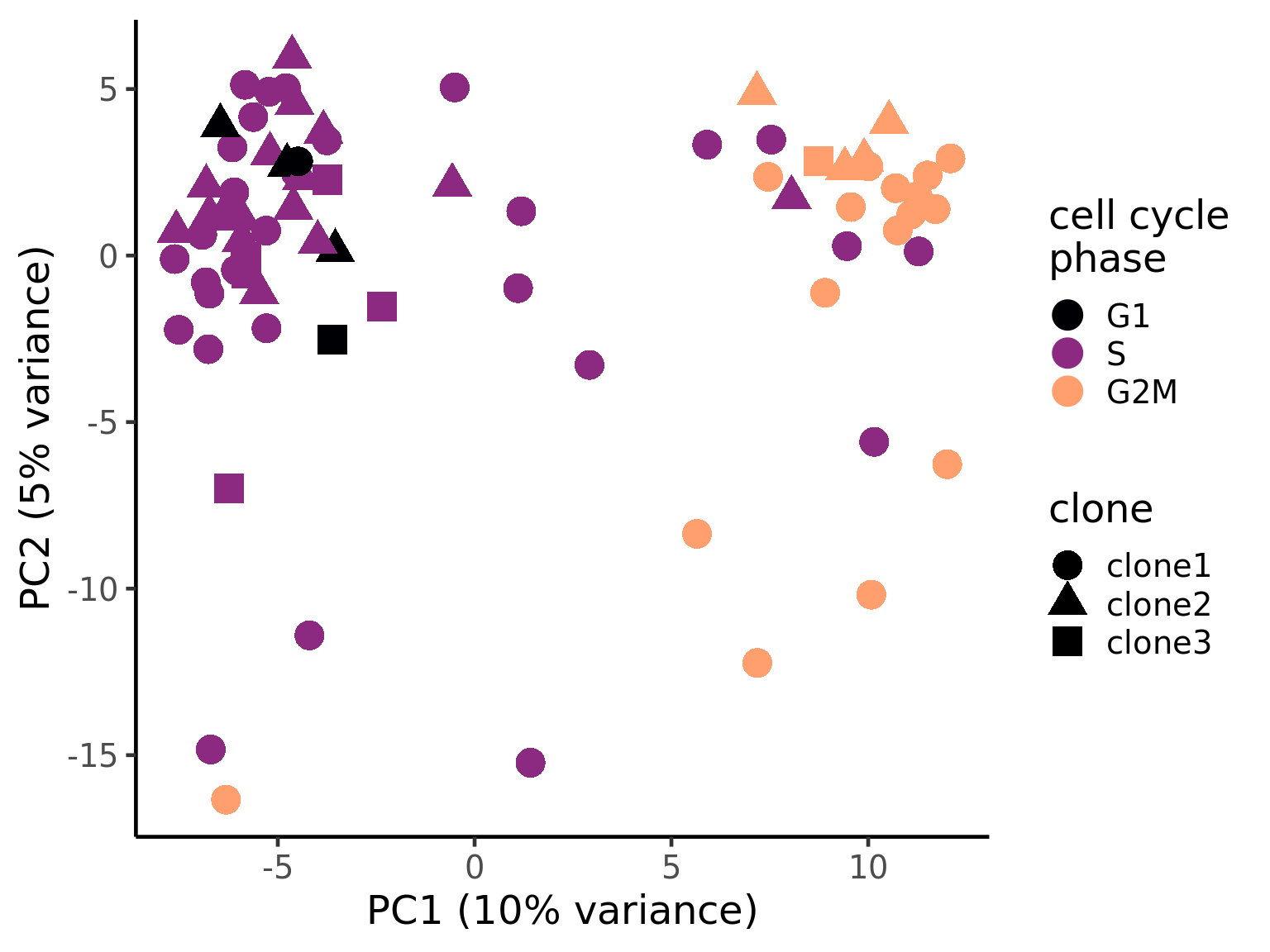
ggsave("figures/donor_specific/carderelax_joxm_pca.png", height = 6, width = 9.5)
ggsave("figures/donor_specific/carderelax_joxm_pca.pdf", height = 6, width = 9.5)
ggsave("figures/donor_specific/carderelax_joxm_pca.svg", height = 6, width = 9.5)


pca_unst$cyclone_phase <- factor(pca_unst$cyclone_phase, levels = c("G1", "S", "G2M"))
ggplot(pca_unst, aes(x = PC2, y = PC3, colour = cyclone_phase,
                     shape = clone)) +
    geom_point(size = 6) +
    scale_color_manual(values = magma(6)[c(1, 3, 5)], name = "cell cycle\nphase") +
    xlab("PC2 (5% variance)") +
    ylab("PC3 (3% variance)") +
    theme_classic(18)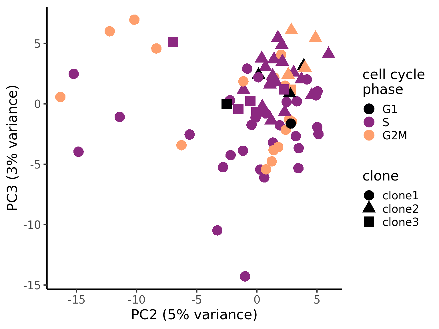
ggplot(pca_unst, aes(x = PC1, y = PC2, fill = G2M,
                     shape = clone)) +
    geom_point(colour = "gray50", size = 5) +
    scale_shape_manual(values = c(21, 23, 25), name = "clone") +
    scico::scale_fill_scico(palette = "bilbao", name  = "G2/M score") +
    scale_size_continuous(range = c(4, 6)) +
    xlab("PC1 (10% variance)") +
    ylab("PC2 (5% variance)") +
    theme_classic(18)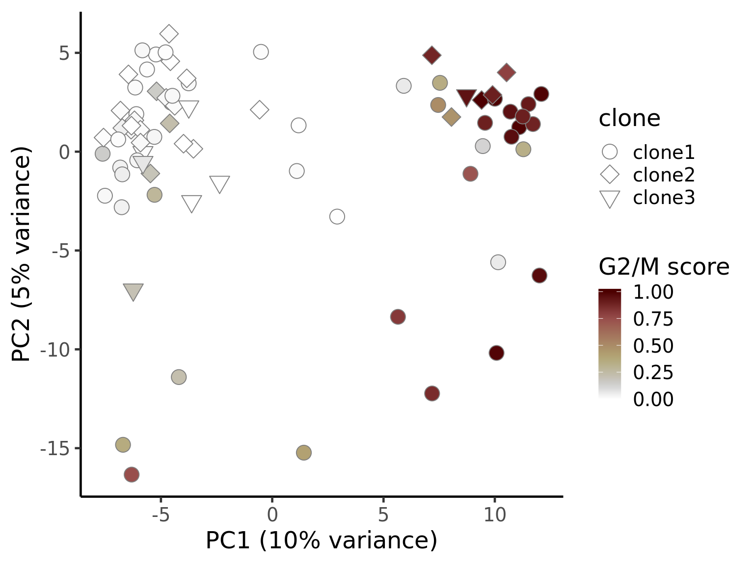
ggsave("figures/donor_specific/carderelax_joxm_pca_g2m_score.png", height = 6, width = 9.5)
ggsave("figures/donor_specific/carderelax_joxm_pca_g2m_score.pdf", height = 6, width = 9.5)
ggsave("figures/donor_specific/carderelax_joxm_pca_g2m_score.svg", height = 6, width = 9.5)

ggplot(pca_unst, aes(x = PC1, y = PC2, colour = S,
                     shape = clone)) +
    geom_point(size = 5) +
    scale_color_viridis(option = "B") +
    xlab("PC1 (10% variance)") +
    ylab("PC2 (5% variance") +
    theme_classic(18)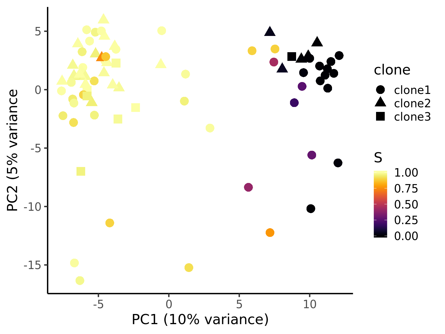
ggplot(pca_unst, aes(x = PC1, y = PC2, colour = G1,
                     shape = clone)) +
    geom_point(size = 5) +
    scale_color_viridis(option = "B") +
    xlab("PC1 (10% variance)") +
    ylab("PC2 (5% variance") +
    theme_classic(18)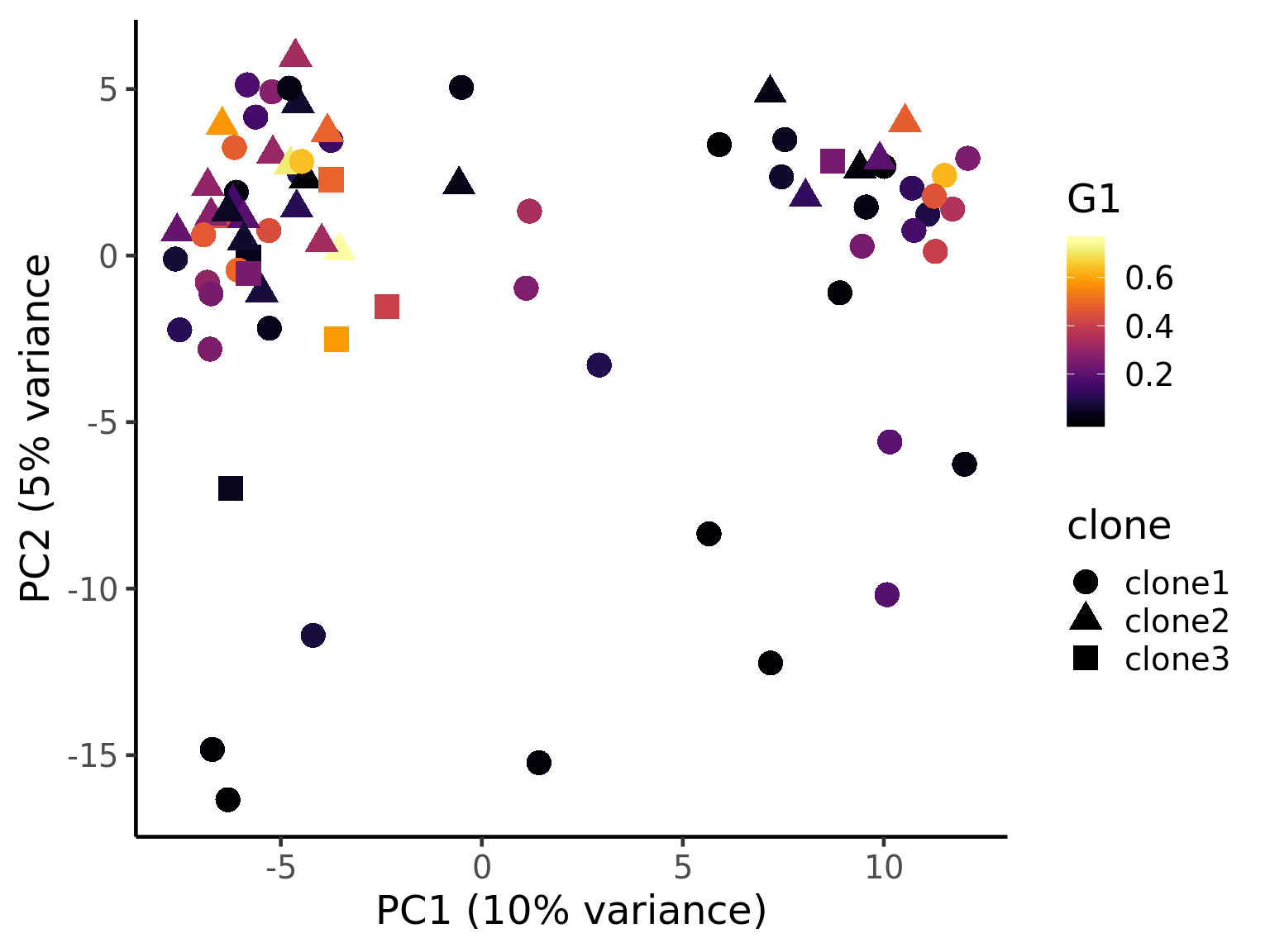
Number of variants used for clone ID looks to have little relationship to global structure in expression PCA space.
ggplot(pca_unst, aes(x = PC1, y = PC2, fill = clone2_prob, size = nvars_cloneid)) +
    geom_point(pch = 21, colour = "gray30") +
    scale_fill_viridis(option = "B", name = "clone2\nprobability") +
    scale_size_continuous(name = "# variants\nfor clone ID") +
    theme_classic(14)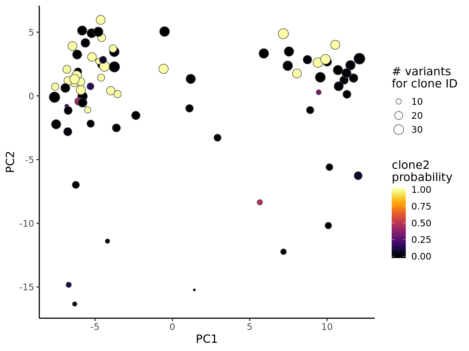
Combined figure
For publication, we put together a combined figure summarising the analyses conducted above.
## tree and cell assignment
fig_tree <- plot_tree(cell_assign_joxm$tree_updated, orient = "v") +
    xlab("Clonal tree") +
    cardelino:::heatmap.theme(size = 16) +
    theme(axis.text.x = element_blank(), axis.title.y = element_text(size = 20))

prob_to_plot <- cell_assign_joxm$prob_mat[
    colnames(sce_joxm)[sce_joxm$well_condition == "unstimulated"], ]
hc <- hclust(dist(prob_to_plot))

clone_ids <- colnames(prob_to_plot)
clone_frac <- colMeans(prob_to_plot[matrixStats::rowMaxs(prob_to_plot) > 0.5,])
clone_perc <- paste0(clone_ids, ": ",
                          round(clone_frac*100, digits = 1), "%")

colnames(prob_to_plot) <- clone_perc
nba.m <- as_data_frame(prob_to_plot[hc$order,]) %>%
    dplyr::mutate(cell = rownames(prob_to_plot[hc$order,])) %>%
    gather(key = "clone", value = "prob", -cell)
nba.m <- dplyr::mutate(nba.m, cell = factor(
    cell, levels = rownames(prob_to_plot[hc$order,])))
fig_assign <- ggplot(nba.m, aes(clone, cell, fill = prob)) +
    geom_tile(show.legend = TRUE) +
    # scale_fill_gradient(low = "white", high = "firebrick4",
    #                     name = "posterior probability of assignment") +
    scico::scale_fill_scico(palette = "oleron", direction = 1) +
    ylab(paste("Single cells")) +
    cardelino:::heatmap.theme(size = 16) + #cardelino:::pub.theme() +
    theme(axis.title.y = element_text(size = 20), legend.position = "bottom",
          legend.text = element_text(size = 12), legend.key.size = unit(0.05, "npc"))

p_tree <- plot_grid(fig_tree, fig_assign, nrow = 2, rel_heights = c(0.46, 0.52))


## cell cycle barplot
p_bar <- as.data.frame(colData(de_res[["sce_list_unst"]][["joxm"]])) %>%
  dplyr::mutate(Cell_Cycle = factor(cyclone_phase, levels = c("G2M", "S", "G1")),
                assigned = factor(assigned, levels = c("clone3", "clone2", "clone1"))) %>%
  ggplot(aes(x = assigned, fill = Cell_Cycle, group = Cell_Cycle)) +
  geom_bar(position = "fill") +
  scale_fill_manual(values = c("#ff6a5c", "#ccdfcb", "#414141")) +
  coord_flip() +
  ylab("proportion of cells") +
  guides(fill = guide_legend(reverse = TRUE)) +
  theme(axis.title.y = element_blank())

## effects on mutated clone
df_to_plot <- mut_genes_df_allcells %>%
  dplyr::filter(!is.na(logFC), donor == "joxm") %>%
  dplyr::filter(!duplicated(gene)) %>%
  dplyr::mutate(
    FDR = p.adjust(PValue, method = "BH"),
    consequence_simplified = factor(
      consequence_simplified,
      levels(as.factor(consequence_simplified))[order(tmp4[["med"]])]),
    de  = ifelse(FDR < 0.2, "FDR < 0.2", "FDR > 0.2"))


p_mutated_clone <- ggplot(df_to_plot, aes(y = logFC, x = consequence_simplified)) +
    geom_hline(yintercept = 0, linetype = 1, colour = "black") +
    geom_boxplot(outlier.size = 0, outlier.alpha = 0, fill = "gray90",
                 colour = "firebrick4", width = 0.2, size = 1) +
    ggbeeswarm::geom_quasirandom(aes(fill = -log10(PValue)),
                                 colour = "gray40", pch = 21, size = 4) +
    geom_segment(aes(y = -0.25, x = 0, yend = -1, xend = 0),
                 colour = "black", size = 1, arrow = arrow(length = unit(0.5, "cm"))) +
    annotate("text", y = -3, x = 0, size = 6, label = "lower in mutated clone") +
    geom_segment(aes(y = 0.25, x = 0, yend = 1, xend = 0),
                 colour = "black", size = 1, arrow = arrow(length = unit(0.5, "cm"))) +
    annotate("text", y = 3, x = 0, size = 6, label = "higher in mutated clone") +
    scale_x_discrete(expand = c(0.1, .05), name = "consequence") +
    scale_y_continuous(expand = c(0.1, 0.1), name = "logFC") +
    expand_limits(x = c(-0.75, 8)) +
    theme_ridges(22) +
    coord_flip() +
    scale_fill_viridis(option = "B", name = "-log10(P)") +
    theme(strip.background = element_rect(fill = "gray90"),
          legend.position = "right") +
    guides(color = FALSE)

## PCA
p_pca <- ggplot(pca_unst, aes(x = PC2, y = PC3, fill = clone,
                     shape = clone)) +
    geom_point(colour = "gray50", size = 5) +
    scale_shape_manual(values = c(21, 23, 25, 22, 24, 26), name = "clone") +
    # scico::scale_fill_scico(palette = "bilbao", name  = "G2/M score") +
    ggthemes::scale_fill_canva(palette = "Surf and turf") +
    scale_size_continuous(range = c(4, 6)) +
    xlab("PC2 (5% variance)") +
    ylab("PC3 (3% variance)") +
    theme_classic(18)

 # ggplot(pca_unst, aes(x = PC2, y = PC3, colour = clone,
 #                     shape = cyclone_phase)) +
 #    geom_point(alpha = 0.9, size = 5) +
 #    scale_shape_manual(values = c(15, 17, 19), name = "clone") +
 #    # scico::scale_fill_scico(palette = "bilbao", name  = "G2/M score") +
 #    ggthemes::scale_color_canva(palette = "Surf and turf") +
 #    scale_size_continuous(range = c(4, 6)) +
 #    xlab("PC2 (5% variance)") +
 #    ylab("PC3 (3% variance)") +
 #    theme_classic(18)

## volcano
de_joxm_cl2_vs_cl1 <- de_res$qlf_pairwise$joxm$clone2_clone1$table
de_joxm_cl2_vs_cl1[["gene"]] <- rownames(de_joxm_cl2_vs_cl1)
de_joxm_cl2_vs_cl1 <- de_joxm_cl2_vs_cl1 %>%
  dplyr::mutate(FDR = adj_pvalues(ihw(PValue ~ logCPM, alpha = 0.1)),
                sig = FDR < 0.1,
                signed_F = sign(logFC) * F)
de_joxm_cl2_vs_cl1[["lab"]] <- ""
int_genes_entrezid <- c(Hs.H$HALLMARK_G2M_CHECKPOINT, Hs.H$HALLMARK_E2F_TARGETS,
                        Hs.H$HALLMARK_MITOTIC_SPINDLE)
mm <- match(int_genes_entrezid, de_joxm_cl2_vs_cl1$entrezid)
mm <- mm[!is.na(mm)]
int_genes_hgnc <- de_joxm_cl2_vs_cl1$hgnc_symbol[mm]
genes_to_label <- (de_joxm_cl2_vs_cl1[["hgnc_symbol"]] %in% int_genes_hgnc &
                     de_joxm_cl2_vs_cl1[["FDR"]] < 0.01)
de_joxm_cl2_vs_cl1[["lab"]][genes_to_label] <-
  de_joxm_cl2_vs_cl1[["hgnc_symbol"]][genes_to_label]
de_joxm_cl2_vs_cl1[["cell_cycle_gene"]] <- (de_joxm_cl2_vs_cl1$entrezid %in%
                                              int_genes_entrezid)

p_volcano <- ggplot(de_joxm_cl2_vs_cl1, aes(x = logFC, y = -log10(PValue),
                                            fill = sig, label = lab)) +
  geom_point(aes(size = sig), pch = 21, colour = "gray40") +
  geom_label_repel(show.legend = FALSE,
                   arrow = arrow(type = "closed", length = unit(0.25, "cm")),
                   nudge_x = 0.2, nudge_y = 0.3, fill = "gray95") +
  geom_segment(aes(x = -1, y = 0, xend = -4, yend = 0),
               colour = "black", size = 1, arrow = arrow(length = unit(0.5, "cm"))) +
  annotate("text", x = -4, y = -0.5, label = "higher in clone1", size = 6) +
  geom_segment(aes(x = 1, y = 0, xend = 4, yend = 0),
               colour = "black", size = 1, arrow = arrow(length = unit(0.5, "cm"))) +
  annotate("text", x = 4, y = -0.5, label = "higher in clone2", size = 6) +
  scale_fill_manual(values = c("gray60", "firebrick"),
                    label = c("N.S.", "FDR < 10%"), name = "") +
  scale_size_manual(values = c(1, 3), guide = FALSE) +
  ylab(expression(-"log"[10](P))) +
  xlab(expression("log"[2](FC))) +
  guides(alpha = FALSE,
         fill = guide_legend(override.aes = list(size = 5))) +
  theme_classic(20) + theme(legend.position = "right")

# ggplot(de_joxm_cl2_vs_cl1, aes(x = logFC, y = -log10(PValue),
#                                fill = cell_cycle_gene, label = lab)) +
#   geom_point(aes(size = sig), pch = 21, colour = "gray40") +
#   geom_point(aes(size = sig), pch = 21, colour = "gray40",
#              data = dplyr::filter(de_joxm_cl2_vs_cl1, cell_cycle_gene)) +
#   geom_label_repel(show.legend = FALSE,
#                    arrow = arrow(type = "closed", length = unit(0.25, "cm")),
#                    nudge_x = 0.2, nudge_y = 0.3, fill = "gray95") +
#   geom_segment(aes(x = -1, y = 0, xend = -4, yend = 0),
#                colour = "black", size = 1, arrow = arrow(length = unit(0.5, "cm"))) +
#   annotate("text", x = -4, y = -0.5, label = "higher in clone1", size = 6) +
#   geom_segment(aes(x = 1, y = 0, xend = 4, yend = 0),
#                colour = "black", size = 1, arrow = arrow(length = unit(0.5, "cm"))) +
#   annotate("text", x = 4, y = -0.5, label = "higher in clone2", size = 6) +
#   scale_fill_manual(values = c("gray60", "firebrick"),
#                     label = c("N.S.", "FDR < 10%"), name = "") +
#   scale_size_manual(values = c(1, 3), guide = FALSE) +
#   guides(alpha = FALSE) +
#   theme_classic(20) + theme(legend.position = "right")

## genesets
cam_H_pw <- de_res$camera$H$joxm$clone2_clone1$logFC
cam_H_pw[["geneset"]] <- rownames(cam_H_pw)
tmp_sig <- rep("FDR > 10%", nrow(cam_H_pw))
tmp_sig[cam_H_pw[["FDR"]] < 0.05] <- "FDR < 5%"
tmp_sig[cam_H_pw[["FDR"]] >= 0.05 & cam_H_pw[["FDR"]] <= 0.1] <- "5% < FDR < 10%"
cam_H_pw[["sig"]] <- factor(tmp_sig, levels = c("FDR > 10%", "5% < FDR < 10%", "FDR < 5%"))
cam_H_pw[["lab"]] <- ""
cam_H_pw[["lab"]][1:3] <-
    cam_H_pw[["geneset"]][1:3]

cam_H_pw <- dplyr::mutate(
    cam_H_pw,
    Direction = gsub("clone4", "clone2", Direction)
)
p_genesets <- cam_H_pw %>%
  ggplot(aes(x = Direction, y = -log10(PValue), colour = sig,
             label = lab)) +
  ggbeeswarm::geom_quasirandom(aes(size = NGenes)) +
  geom_label_repel(show.legend = FALSE,
                   nudge_y = 0.3, nudge_x = 0.3, fill = "gray95") +
  scale_colour_manual(values = c("gray50", "darkorange2", "firebrick"),
                      name = "") +
  guides(alpha = FALSE,
         colour = guide_legend(override.aes = list(size = 5))) +
  xlab("Gene set enrichment direction") +
  ylab(expression(-"log"[10](P))) +
  theme_classic(20) + theme(legend.position = "right")


## produce combined fig
## combine pca and barplot
p_bar_pca <- ggdraw() +
  draw_plot(p_pca + theme(legend.justification = "top"), 0, 0, 1, 1) +
  draw_plot(p_bar, x = 0.48, 0.1, height = 0.35, width = 0.52, scale = 1)

pp <- ggdraw() +
    draw_plot(p_tree, x = 0,  y = 0.45, width = 0.48, height = 0.55, scale = 1) +
    draw_plot(p_bar_pca, x = 0.52, y = 0.45, width = 0.48, height = 0.55, scale = 1) +
    draw_plot(p_volcano, x = 0,  y = 0, width = 0.48, height = 0.45, scale = 1) +
    draw_plot(p_genesets, x = 0.52,  y = 0, width = 0.48, height = 0.45, scale = 1) +
    draw_plot_label(letters[1:4], x = c(0, 0.5, 0, 0.5),
                    y = c(1, 1, 0.45, 0.45), size = 36)

ggsave("figures/donor_specific/carderelax_joxm_combined_fig.png",
       height = 16, width = 18, plot = pp)
ggsave("figures/donor_specific/carderelax_joxm_combined_fig.pdf",
       height = 16, width = 18, plot = pp)


## plots for talk
ggsave("figures/donor_specific/carderelax_joxm_bar_pca.png", plot = p_bar_pca,
       height = 7, width = 10)
ggsave("figures/donor_specific/carderelax_joxm_volcano.png", plot = p_volcano,
       height = 6, width = 10)
ggsave("figures/donor_specific/carderelax_joxm_genesets.png", plot = p_genesets,
       height = 6, width = 10)
ggsave("figures/donor_specific/carderelax_joxm_mutated_clone.png", plot = p_mutated_clone,
       height = 6, width = 14)

pp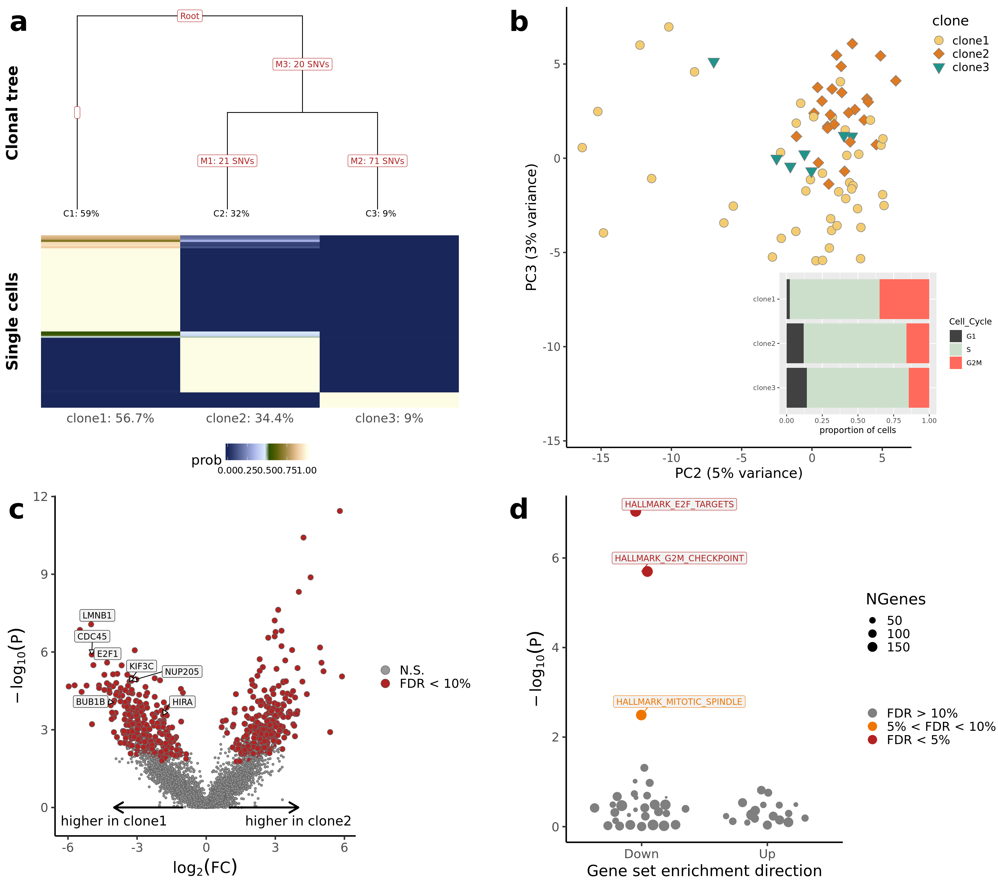
# ggdraw() +
#     draw_plot(p_tree, x = 0,  y = 0.57, width = 0.48, height = 0.43, scale = 1) +
#     draw_plot(p_bar_pca, x = 0.52, y = 0.57, width = 0.48, height = 0.43, scale = 1) +
#     draw_plot(p_volcano, x = 0,  y = 0.3, width = 0.48, height = 0.27, scale = 1) +
#     draw_plot(p_genesets, x = 0.52,  y = 0.3, width = 0.48, height = 0.27, scale = 1) +
#     #draw_plot(p_table, x = 0,  y = 0.2, width = 1, height = 0.15, scale = 1) +
#     draw_plot(p_mutated_clone, x = 0.05,  y = 0, width = 0.9, height = 0.3, scale = 1) +
#     draw_plot_label(letters[1:5], x = c(0, 0.5, 0, 0.5, 0),
#                     y = c(1, 1, 0.57, 0.57, 0.3), size = 36)
# ggsave("figures/donor_specific/joxm_combined_fig.png",
#        height = 20, width = 19)
# ggsave("figures/donor_specific/joxm_combined_fig.pdf",
#        height = 20, width = 19)
─ Session info ──────────────────────────────────────────────────────────
 setting  value
 version  R version 3.6.0 (2019-04-26)
 os       Ubuntu 18.04.3 LTS
 system   x86_64, linux-gnu
 ui       X11
 language (EN)
 collate  en_AU.UTF-8
 ctype    en_AU.UTF-8
 tz       Australia/Melbourne
 date     2019-10-30

─ Packages ──────────────────────────────────────────────────────────────
 package              * version   date       lib
 AnnotationDbi        * 1.46.1    2019-08-20 [1]
 ape                    5.3       2019-03-17 [1]
 assertthat             0.2.1     2019-03-21 [1]
 backports              1.1.4     2019-04-10 [1]
 beeswarm               0.2.3     2016-04-25 [1]
 Biobase              * 2.44.0    2019-05-02 [1]
 BiocGenerics         * 0.30.0    2019-05-02 [1]
 BiocNeighbors          1.2.0     2019-05-02 [1]
 BiocParallel         * 1.18.1    2019-08-06 [1]
 BiocSingular           1.0.0     2019-05-02 [1]
 biomaRt                2.40.4    2019-08-19 [1]
 Biostrings             2.52.0    2019-05-02 [1]
 bit                    1.1-14    2018-05-29 [1]
 bit64                  0.9-7     2017-05-08 [1]
 bitops                 1.0-6     2013-08-17 [1]
 blob                   1.2.0     2019-07-09 [1]
 broom                  0.5.2     2019-04-07 [1]
 BSgenome               1.52.0    2019-05-02 [1]
 callr                  3.3.2     2019-09-22 [1]
 cardelino            * 0.6.4     2019-08-21 [1]
 cellranger             1.1.0     2016-07-27 [1]
 cli                    1.1.0     2019-03-19 [1]
 colorspace             1.4-1     2019-03-18 [1]
 cowplot              * 1.0.0     2019-07-11 [1]
 crayon                 1.3.4     2017-09-16 [1]
 DBI                    1.0.0     2018-05-02 [1]
 DelayedArray         * 0.10.0    2019-05-02 [1]
 DelayedMatrixStats     1.6.1     2019-09-08 [1]
 desc                   1.2.0     2018-05-01 [1]
 devtools               2.2.1     2019-09-24 [1]
 digest                 0.6.21    2019-09-20 [1]
 dplyr                * 0.8.3     2019-07-04 [1]
 edgeR                * 3.26.8    2019-09-01 [1]
 ellipsis               0.3.0     2019-09-20 [1]
 evaluate               0.14      2019-05-28 [1]
 fansi                  0.4.0     2018-10-05 [1]
 farver                 1.1.0     2018-11-20 [1]
 fdrtool                1.2.15    2015-07-08 [1]
 forcats              * 0.4.0     2019-02-17 [1]
 fs                     1.3.1     2019-05-06 [1]
 gdtools              * 0.2.0     2019-09-03 [1]
 generics               0.0.2     2018-11-29 [1]
 GenomeInfoDb         * 1.20.0    2019-05-02 [1]
 GenomeInfoDbData       1.2.1     2019-04-30 [1]
 GenomicAlignments      1.20.1    2019-06-18 [1]
 GenomicFeatures        1.36.4    2019-07-10 [1]
 GenomicRanges        * 1.36.1    2019-09-06 [1]
 ggbeeswarm             0.6.0     2017-08-07 [1]
 ggforce              * 0.3.1     2019-08-20 [1]
 ggplot2              * 3.2.1     2019-08-10 [1]
 ggrepel              * 0.8.1     2019-05-07 [1]
 ggridges             * 0.5.1     2018-09-27 [1]
 ggthemes             * 4.2.0     2019-05-13 [1]
 ggtree                 1.16.6    2019-08-26 [1]
 git2r                  0.26.1    2019-06-29 [1]
 glue                   1.3.1     2019-03-12 [1]
 gridExtra              2.3       2017-09-09 [1]
 gtable                 0.3.0     2019-03-25 [1]
 haven                  2.1.1     2019-07-04 [1]
 hms                    0.5.1     2019-08-23 [1]
 htmltools              0.3.6     2017-04-28 [1]
 httr                   1.4.1     2019-08-05 [1]
 IHW                  * 1.12.0    2019-05-02 [1]
 IRanges              * 2.18.3    2019-09-24 [1]
 irlba                  2.3.3     2019-02-05 [1]
 jsonlite               1.6       2018-12-07 [1]
 knitr                  1.25      2019-09-18 [1]
 labeling               0.3       2014-08-23 [1]
 lattice                0.20-38   2018-11-04 [4]
 lazyeval               0.2.2     2019-03-15 [1]
 lifecycle              0.1.0     2019-08-01 [1]
 limma                * 3.40.6    2019-07-26 [1]
 locfit                 1.5-9.1   2013-04-20 [1]
 lpsymphony             1.12.0    2019-05-02 [1]
 lubridate              1.7.4     2018-04-11 [1]
 magrittr               1.5       2014-11-22 [1]
 MASS                   7.3-51.1  2018-11-01 [4]
 Matrix                 1.2-17    2019-03-22 [1]
 matrixStats          * 0.55.0    2019-09-07 [1]
 memoise                1.1.0     2017-04-21 [1]
 modelr                 0.1.5     2019-08-08 [1]
 munsell                0.5.0     2018-06-12 [1]
 nlme                   3.1-139   2019-04-09 [4]
 org.Hs.eg.db         * 3.8.2     2019-05-01 [1]
 pheatmap               1.0.12    2019-01-04 [1]
 pillar                 1.4.2     2019-06-29 [1]
 pkgbuild               1.0.5     2019-08-26 [1]
 pkgconfig              2.0.3     2019-09-22 [1]
 pkgload                1.0.2     2018-10-29 [1]
 plyr                   1.8.4     2016-06-08 [1]
 polyclip               1.10-0    2019-03-14 [1]
 prettyunits            1.0.2     2015-07-13 [1]
 processx               3.4.1     2019-07-18 [1]
 progress               1.2.2     2019-05-16 [1]
 ps                     1.3.0     2018-12-21 [1]
 purrr                * 0.3.2     2019-03-15 [1]
 R6                     2.4.0     2019-02-14 [1]
 RColorBrewer         * 1.1-2     2014-12-07 [1]
 Rcpp                   1.0.2     2019-07-25 [1]
 RCurl                  1.95-4.12 2019-03-04 [1]
 readr                * 1.3.1     2018-12-21 [1]
 readxl                 1.3.1     2019-03-13 [1]
 remotes                2.1.0     2019-06-24 [1]
 rlang                * 0.4.0     2019-06-25 [1]
 rmarkdown              1.15      2019-08-21 [1]
 rprojroot              1.3-2     2018-01-03 [1]
 Rsamtools              2.0.1     2019-09-19 [1]
 RSQLite                2.1.2     2019-07-24 [1]
 rstudioapi             0.10      2019-03-19 [1]
 rsvd                   1.0.2     2019-07-29 [1]
 rtracklayer            1.44.4    2019-09-06 [1]
 rvcheck                0.1.3     2018-12-06 [1]
 rvest                  0.3.4     2019-05-15 [1]
 S4Vectors            * 0.22.1    2019-09-09 [1]
 scales                 1.0.0     2018-08-09 [1]
 scater               * 1.12.2    2019-05-24 [1]
 scico                  1.1.0     2018-11-20 [1]
 sessioninfo            1.1.1     2018-11-05 [1]
 SingleCellExperiment * 1.6.0     2019-05-02 [1]
 slam                   0.1-45    2019-02-26 [1]
 snpStats               1.34.0    2019-05-02 [1]
 stringi                1.4.3     2019-03-12 [1]
 stringr              * 1.4.0     2019-02-10 [1]
 SummarizedExperiment * 1.14.1    2019-07-31 [1]
 superheat            * 0.1.0     2017-02-04 [1]
 survival               2.43-3    2018-11-26 [4]
 svglite                1.2.2     2019-05-17 [1]
 systemfonts            0.1.1     2019-07-01 [1]
 testthat               2.2.1     2019-07-25 [1]
 tibble               * 2.1.3     2019-06-06 [1]
 tidyr                * 1.0.0     2019-09-11 [1]
 tidyselect             0.2.5     2018-10-11 [1]
 tidytree               0.2.7     2019-09-12 [1]
 tidyverse            * 1.2.1     2017-11-14 [1]
 treeio                 1.8.2     2019-08-21 [1]
 tweenr                 1.0.1     2018-12-14 [1]
 usethis                1.5.1     2019-07-04 [1]
 utf8                   1.1.4     2018-05-24 [1]
 VariantAnnotation      1.30.1    2019-05-19 [1]
 vctrs                  0.2.0     2019-07-05 [1]
 vipor                  0.4.5     2017-03-22 [1]
 viridis              * 0.5.1     2018-03-29 [1]
 viridisLite          * 0.3.0     2018-02-01 [1]
 whisker                0.4       2019-08-28 [1]
 withr                  2.1.2     2018-03-15 [1]
 workflowr              1.4.0     2019-06-08 [1]
 xfun                   0.9       2019-08-21 [1]
 XML                    3.98-1.20 2019-06-06 [1]
 xml2                   1.2.2     2019-08-09 [1]
 XVector                0.24.0    2019-05-02 [1]
 yaml                   2.2.0     2018-07-25 [1]
 zeallot                0.1.0     2018-01-28 [1]
 zlibbioc               1.30.0    2019-05-02 [1]
 source
 Bioconductor
 CRAN (R 3.6.0)
 CRAN (R 3.6.0)
 CRAN (R 3.6.0)
 CRAN (R 3.6.0)
 Bioconductor
 Bioconductor
 Bioconductor
 Bioconductor
 Bioconductor
 Bioconductor
 Bioconductor
 CRAN (R 3.6.0)
 CRAN (R 3.6.0)
 CRAN (R 3.6.0)
 CRAN (R 3.6.0)
 CRAN (R 3.6.0)
 Bioconductor
 CRAN (R 3.6.0)
 Github (PMBio/cardelino@efd846f)
 CRAN (R 3.6.0)
 CRAN (R 3.6.0)
 CRAN (R 3.6.0)
 CRAN (R 3.6.0)
 CRAN (R 3.6.0)
 CRAN (R 3.6.0)
 Bioconductor
 Bioconductor
 CRAN (R 3.6.0)
 CRAN (R 3.6.0)
 CRAN (R 3.6.0)
 CRAN (R 3.6.0)
 Bioconductor
 CRAN (R 3.6.0)
 CRAN (R 3.6.0)
 CRAN (R 3.6.0)
 CRAN (R 3.6.0)
 CRAN (R 3.6.0)
 CRAN (R 3.6.0)
 CRAN (R 3.6.0)
 CRAN (R 3.6.0)
 CRAN (R 3.6.0)
 Bioconductor
 Bioconductor
 Bioconductor
 Bioconductor
 Bioconductor
 CRAN (R 3.6.0)
 CRAN (R 3.6.0)
 CRAN (R 3.6.0)
 CRAN (R 3.6.0)
 CRAN (R 3.6.0)
 CRAN (R 3.6.0)
 Bioconductor
 CRAN (R 3.6.0)
 CRAN (R 3.6.0)
 CRAN (R 3.6.0)
 CRAN (R 3.6.0)
 CRAN (R 3.6.0)
 CRAN (R 3.6.0)
 CRAN (R 3.6.0)
 CRAN (R 3.6.0)
 Bioconductor
 Bioconductor
 CRAN (R 3.6.0)
 CRAN (R 3.6.0)
 CRAN (R 3.6.0)
 CRAN (R 3.6.0)
 CRAN (R 3.5.1)
 CRAN (R 3.6.0)
 CRAN (R 3.6.0)
 Bioconductor
 CRAN (R 3.6.0)
 Bioconductor (R 3.6.0)
 CRAN (R 3.6.0)
 CRAN (R 3.6.0)
 CRAN (R 3.5.1)
 CRAN (R 3.6.0)
 CRAN (R 3.6.0)
 CRAN (R 3.6.0)
 CRAN (R 3.6.0)
 CRAN (R 3.6.0)
 CRAN (R 3.5.3)
 Bioconductor
 CRAN (R 3.6.0)
 CRAN (R 3.6.0)
 CRAN (R 3.6.0)
 CRAN (R 3.6.0)
 CRAN (R 3.6.0)
 CRAN (R 3.6.0)
 CRAN (R 3.6.0)
 CRAN (R 3.6.0)
 CRAN (R 3.6.0)
 CRAN (R 3.6.0)
 CRAN (R 3.6.0)
 CRAN (R 3.6.0)
 CRAN (R 3.6.0)
 CRAN (R 3.6.0)
 CRAN (R 3.6.0)
 CRAN (R 3.6.0)
 CRAN (R 3.6.0)
 CRAN (R 3.6.0)
 CRAN (R 3.6.0)
 CRAN (R 3.6.0)
 CRAN (R 3.6.0)
 CRAN (R 3.6.0)
 Bioconductor
 CRAN (R 3.6.0)
 CRAN (R 3.6.0)
 CRAN (R 3.6.0)
 Bioconductor
 CRAN (R 3.6.0)
 CRAN (R 3.6.0)
 Bioconductor
 CRAN (R 3.6.0)
 Bioconductor
 CRAN (R 3.6.0)
 CRAN (R 3.6.0)
 Bioconductor
 CRAN (R 3.6.0)
 Bioconductor
 CRAN (R 3.6.0)
 CRAN (R 3.6.0)
 Bioconductor
 CRAN (R 3.6.0)
 CRAN (R 3.5.1)
 CRAN (R 3.6.0)
 CRAN (R 3.6.0)
 CRAN (R 3.6.0)
 CRAN (R 3.6.0)
 CRAN (R 3.6.0)
 CRAN (R 3.6.0)
 CRAN (R 3.6.0)
 CRAN (R 3.6.0)
 Bioconductor
 CRAN (R 3.6.0)
 CRAN (R 3.6.0)
 CRAN (R 3.6.0)
 Bioconductor
 CRAN (R 3.6.0)
 CRAN (R 3.6.0)
 CRAN (R 3.6.0)
 CRAN (R 3.6.0)
 CRAN (R 3.6.0)
 CRAN (R 3.6.0)
 CRAN (R 3.6.0)
 CRAN (R 3.6.0)
 CRAN (R 3.6.0)
 CRAN (R 3.6.0)
 Bioconductor
 CRAN (R 3.6.0)
 CRAN (R 3.6.0)
 Bioconductor

[1] /home/AD.SVI.EDU.AU/dmccarthy/R/x86_64-pc-linux-gnu-library/3.6
[2] /usr/local/lib/R/site-library
[3] /usr/lib/R/site-library
[4] /usr/lib/R/library