Overview of lines
Raghd Rostom, Daniel J. Kunz & Davis J. McCarthy
Last updated: 2019-10-30
Checks: 7 0
Knit directory: fibroblast-clonality/
This reproducible R Markdown analysis was created with workflowr (version 1.4.0). The Checks tab describes the reproducibility checks that were applied when the results were created. The Past versions tab lists the development history.
Great! Since the R Markdown file has been committed to the Git repository, you know the exact version of the code that produced these results.
Great job! The global environment was empty. Objects defined in the global environment can affect the analysis in your R Markdown file in unknown ways. For reproduciblity it’s best to always run the code in an empty environment.
The command set.seed(20180807) was run prior to running the code in the R Markdown file. Setting a seed ensures that any results that rely on randomness, e.g. subsampling or permutations, are reproducible.
Great job! Recording the operating system, R version, and package versions is critical for reproducibility.
Nice! There were no cached chunks for this analysis, so you can be confident that you successfully produced the results during this run.
Great job! Using relative paths to the files within your workflowr project makes it easier to run your code on other machines.
Great! You are using Git for version control. Tracking code development and connecting the code version to the results is critical for reproducibility. The version displayed above was the version of the Git repository at the time these results were generated.
Note that you need to be careful to ensure that all relevant files for the analysis have been committed to Git prior to generating the results (you can use wflow_publish or wflow_git_commit). workflowr only checks the R Markdown file, but you know if there are other scripts or data files that it depends on. Below is the status of the Git repository when the results were generated:
Ignored files:
    Ignored:    .DS_Store
    Ignored:    .Rhistory
    Ignored:    .Rproj.user/
    Ignored:    .vscode/
    Ignored:    analysis/figure/
    Ignored:    code/.DS_Store
    Ignored:    code/selection/.DS_Store
    Ignored:    code/selection/.Rhistory
    Ignored:    code/selection/figures/
    Ignored:    data/.DS_Store
    Ignored:    logs/
    Ignored:    src/.DS_Store
    Ignored:    src/Rmd/.Rhistory

Untracked files:
    Untracked:  .dockerignore
    Untracked:  .dropbox
    Untracked:  .snakemake/
    Untracked:  Rplots.pdf
    Untracked:  Snakefile_clonality
    Untracked:  Snakefile_somatic_calling
    Untracked:  analysis/.ipynb_checkpoints/
    Untracked:  analysis/assess_mutect2_fibro-ipsc_variant_calls.ipynb
    Untracked:  analysis/cardelino_fig1b.R
    Untracked:  analysis/cardelino_fig2b.R
    Untracked:  code/analysis_for_garx.Rmd
    Untracked:  code/selection/data/
    Untracked:  code/selection/fit-dist.nb
    Untracked:  code/selection/result-figure.R
    Untracked:  code/yuanhua/
    Untracked:  data/Melanoma-RegevGarraway-DFCI-scRNA-Seq/
    Untracked:  data/PRJNA485423/
    Untracked:  data/canopy/
    Untracked:  data/cell_assignment/
    Untracked:  data/cnv/
    Untracked:  data/de_analysis_FTv62/
    Untracked:  data/donor_info_070818.txt
    Untracked:  data/donor_info_core.csv
    Untracked:  data/donor_neutrality.tsv
    Untracked:  data/exome-point-mutations/
    Untracked:  data/fdr10.annot.txt.gz
    Untracked:  data/human_H_v5p2.rdata
    Untracked:  data/human_c2_v5p2.rdata
    Untracked:  data/human_c6_v5p2.rdata
    Untracked:  data/neg-bin-rsquared-petr.csv
    Untracked:  data/neutralitytestr-petr.tsv
    Untracked:  data/raw/
    Untracked:  data/sce_merged_donors_cardelino_donorid_all_qc_filt.rds
    Untracked:  data/sce_merged_donors_cardelino_donorid_all_with_qc_labels.rds
    Untracked:  data/sce_merged_donors_cardelino_donorid_unstim_qc_filt.rds
    Untracked:  data/sces/
    Untracked:  data/selection/
    Untracked:  data/simulations/
    Untracked:  data/variance_components/
    Untracked:  figures/
    Untracked:  output/differential_expression/
    Untracked:  output/differential_expression_cardelino-relax/
    Untracked:  output/donor_specific/
    Untracked:  output/line_info.tsv
    Untracked:  output/nvars_by_category_by_donor.tsv
    Untracked:  output/nvars_by_category_by_line.tsv
    Untracked:  output/variance_components/
    Untracked:  qolg_BIC.pdf
    Untracked:  references/
    Untracked:  reports/
    Untracked:  src/Rmd/DE_pathways_FTv62_callset_clones_pairwise_vs_base.unst_cells.carderelax.Rmd
    Untracked:  src/Rmd/Rplots.pdf
    Untracked:  src/Rmd/cell_assignment_cardelino-relax_template.Rmd
    Untracked:  tree.txt
Note that any generated files, e.g. HTML, png, CSS, etc., are not included in this status report because it is ok for generated content to have uncommitted changes.
These are the previous versions of the R Markdown and HTML files. If you’ve configured a remote Git repository (see ?wflow_git_remote), click on the hyperlinks in the table below to view them.
| File | Version | Author | Date | Message |
|---|---|---|---|---|
| Rmd | cf8eb55 | Davis McCarthy | 2019-10-30 | Fixing bugs in overview_lines |
| Rmd | ff03735 | Davis McCarthy | 2019-10-30 | Merge branch ‘master’ of https://github.com/davismcc/fibroblast-clonality |
| Rmd | 550176f | Davis McCarthy | 2019-10-30 | Updating analysis to reflect accepted ms |
| html | 8729e02 | davismcc | 2018-11-09 | Build site. |
| Rmd | 3c39fc2 | d-j-k | 2018-11-01 | updated selection analysis |
| html | 0540cdb | davismcc | 2018-09-02 | Build site. |
| Rmd | f5a4631 | davismcc | 2018-09-02 | Final plot tweaks |
| html | f0ed980 | davismcc | 2018-08-31 | Build site. |
| Rmd | 1310c93 | davismcc | 2018-08-30 | Tweaking plots |
| Rmd | 846dec4 | davismcc | 2018-08-29 | Some small tweaks/additions to analyses |
| html | ca3438f | davismcc | 2018-08-29 | Build site. |
| Rmd | dc78a95 | davismcc | 2018-08-29 | Minor updates to analyses. |
| html | e573f2f | davismcc | 2018-08-27 | Build site. |
| html | 9ec2a59 | davismcc | 2018-08-26 | Build site. |
| html | 36acf15 | davismcc | 2018-08-25 | Build site. |
| Rmd | d618fe5 | davismcc | 2018-08-25 | Updating analyses |
| html | 090c1b9 | davismcc | 2018-08-24 | Build site. |
| html | 8f884ae | davismcc | 2018-08-24 | Adding data pre-processing and line overview html files |
| Rmd | 5aa174b | davismcc | 2018-08-20 | Tidying up and saving dataframe to output file |
| Rmd | fc582db | davismcc | 2018-08-20 | Fixing up small bug. |
| Rmd | 3856e54 | davismcc | 2018-08-20 | Adding overview analysis of lines |
This document provides overview information for 32 healthy human fibroblast cell lines used in this project. Note that each cell line was each derived from a distinct donor, so we use the terms “line” and “donor” interchangeably.
Load libraries and data
library(readr)
library(dplyr)
library(scran)
library(scater)
library(viridis)
library(ggplot2)
library(ggforce)
library(ggridges)
library(SingleCellExperiment)
library(edgeR)
library(limma)
library(org.Hs.eg.db)
library(cowplot)
library(gplots)
library(ggrepel)
library(sigfit)
library(Rcpp)
library(deconstructSigs)
options(stringsAsFactors = FALSE)
Load donor level information.
donor_info <- as.data.frame(read_csv("data/donor_info_core.csv"))
# merge age bins
donor_info$age_decade <- ""
for (i in 1:nrow(donor_info)) {
  if (donor_info$age[i] %in% c("30-34", "35-39"))
    donor_info$age_decade[i] <- "30-39"
  if (donor_info$age[i] %in% c("40-44", "45-49"))
    donor_info$age_decade[i] <- "40-49"
  if (donor_info$age[i] %in% c("50-54", "55-59"))
    donor_info$age_decade[i] <- "50-59"
  if (donor_info$age[i] %in% c("60-64", "65-69"))
    donor_info$age_decade[i] <- "60-69"
  if (donor_info$age[i] %in% c("70-74", "75-79"))
    donor_info$age_decade[i] <- "70-79"
}
Load exome variant sites.
exome_sites <- read_tsv("data/exome-point-mutations/high-vs-low-exomes.v62.ft.filt_lenient-alldonors.txt.gz",
                        col_types = "ciccdcciiiiccccccccddcdcll", comment = "#",
                        col_names = TRUE)
exome_sites <- dplyr::mutate(
  exome_sites,
  chrom = paste0("chr", gsub("chr", "", chrom)),
  var_id = paste0(chrom, ":", pos, "_", ref, "_", alt),
  chr_pos = paste0(chrom, "_", pos))

exome_sites <- as.data.frame(exome_sites)
## deduplicate sites list
exome_sites <- exome_sites[!duplicated(exome_sites[["var_id"]]),]
## calculate coverage at sites for each donor
donor_vars_coverage <- list()
for (i in unique(exome_sites$donor_short_id)) {
  exome_sites_subset <- exome_sites[exome_sites$donor_short_id == i, ]
  donor_vars_coverage[[i]] <- exome_sites_subset$nREF_fibro + exome_sites_subset$nALT_fibro
}
Load VEP annotations and show table with number of variants assigned to each functional annotation category.
vep_best <- read_tsv("data/exome-point-mutations/high-vs-low-exomes.v62.ft.alldonors-filt_lenient.all_filt_sites.vep_most_severe_csq.txt")
colnames(vep_best)[1] <- "Uploaded_variation"
## deduplicate dataframe
vep_best <- as.data.frame(vep_best[!duplicated(vep_best[["Uploaded_variation"]]),])
as.data.frame(table(vep_best[["Consequence"]]))
Var1 Freq
1 3_prime_UTR_variant 181
2 5_prime_UTR_variant 121
3 downstream_gene_variant 13
4 intergenic_variant 13
5 intron_variant 1539
6 mature_miRNA_variant 3
7 missense_variant 3648
8 non_coding_transcript_exon_variant 428
9 regulatory_region_variant 1
10 splice_acceptor_variant 41
11 splice_donor_variant 24
12 splice_region_variant 291
13 start_lost 9
14 stop_gained 227
15 stop_lost 2
16 stop_retained_variant 5
17 synonymous_variant 1923
18 upstream_gene_variant 34Add consequences to exome sites.
vep_best[["var_id"]] <- paste0("chr", vep_best[["Uploaded_variation"]])
exome_sites <- inner_join(exome_sites,
                          vep_best[, c("var_id", "Location", "Consequence")],
                          by = "var_id")
Add donor level mutation information (aggregate across impacts) Not used in manuscript, but still calculated to store in donor_info table.
impactful_csq <- c("stop_lost", "start_lost", "stop_gained",
                   "splice_donor_variant", "splice_acceptor_variant",
                   "splice_region_variant", "missense_variant")
donor_info$num_mutations <- NA
donor_info$num_synonymous <- NA
donor_info$num_missense <- NA
donor_info$num_splice_region <- NA
donor_info$num_splice_acceptor <- NA
donor_info$num_splice_donor <- NA
donor_info$num_stop_gained <- NA
donor_info$num_start_lost <- NA
donor_info$num_stop_lost <- NA
for (i in unique(donor_info$donor_short)) {
  if (i %in% unique(exome_sites$donor_short_id)) {
    exome_sites_subset <- exome_sites[exome_sites$donor_short_id == i, ]
    donor_info$num_mutations[donor_info$donor_short == i] <- length(exome_sites_subset$Consequence)
    donor_info$num_synonymous[donor_info$donor_short == i] <- sum(exome_sites_subset$Consequence == "synonymous_variant")
    donor_info$num_missense[donor_info$donor_short == i] <- sum(exome_sites_subset$Consequence == "missense_variant")
    donor_info$num_splice_region[donor_info$donor_short == i] <- sum(exome_sites_subset$Consequence == "splice_region_variant")
    donor_info$num_splice_acceptor[donor_info$donor_short == i] <- sum(exome_sites_subset$Consequence == "splice_acceptor_variant")
    donor_info$num_splice_donor[donor_info$donor_short == i] <- sum(exome_sites_subset$Consequence == "splice_donor_variant")
    donor_info$num_stop_gained[donor_info$donor_short == i] <- sum(exome_sites_subset$Consequence == "stop_gained")
    donor_info$num_start_lost[donor_info$donor_short == i] <- sum(exome_sites_subset$Consequence == "start_lost")
    donor_info$num_stop_lost[donor_info$donor_short == i] <- sum(exome_sites_subset$Consequence == "stop_lost")
  }
}
Mutational signatures
Add donor level mutation signature exposures, using the sigfit package and 30 COSMIC signatures. We load the filtered exome variant sites and calculate the tri-nucleotide context for each variant (required for computing signature exposures), using a function from the deconstructSigs package.
data("cosmic_signatures", package = "sigfit")

##new input
mutation_list <- read.table("data/exome-point-mutations/high-vs-low-exomes.v62.ft.filt_lenient-alldonors.txt.gz", header = TRUE)
mutation_list$chr_pos <- paste0("chr", mutation_list$chr, "_", mutation_list$pos)

mutation_donors <- unique(mutation_list$donor_short_id)
mutation_list_donors <- list()
for (i in mutation_donors) {
  cat("....reading ", i, "\n")
  mutation_list_donors[[i]] <- mutation_list[which(mutation_list$donor_short_id == i),]
  mutation_list_donors[[i]]$chr <- paste0("chr", mutation_list_donors[[i]]$chrom)
  mutation_list_donors[[i]]$chr_pos = paste0(mutation_list_donors[[i]]$chr, "_", mutation_list_donors[[i]]$pos)
}

## Calculate triNucleotide contexts for mutations using deconstructSigs command
mut_triNs <- list()
for (i in mutation_donors) {
  cat("....processing ", i, "\n")
  mut_triNs[[i]] <- mut.to.sigs.input(mutation_list_donors[[i]], sample.id = "donor_short_id",
                                      chr = "chr", pos = "pos", ref = "ref", alt = "alt")
}

## Convert to correct format
sig_triNs <- character()
for (j in 1:96) {
  c1 <- substr(colnames(mut_triNs[[1]])[j], 1,1)
  ref <- substr(colnames(mut_triNs[[1]])[j], 3,3)
  alt <- substr(colnames(mut_triNs[[1]])[j], 5,5)
  c3 <- substr(colnames(mut_triNs[[1]])[j], 7,7)
  triN_sigfit <- paste0(c1,ref,c3,">",c1,alt,c3)
  sig_triNs[j] <- triN_sigfit
}

for (i in mutation_donors) {
  colnames(mut_triNs[[i]]) <- sig_triNs
}

## Fit signatures using sigfit
mcmc_samples_fit <- list()
set.seed(1234)
for (i in mutation_donors) {
  mcmc_samples_fit[[i]] <- sigfit::fit_signatures(
    counts = mut_triNs[[i]], signatures = cosmic_signatures,
    iter = 2000, warmup = 1000, chains = 1, seed = 1)
}

## Estimate exposures using sigfit
exposures <- list()
for (i in mutation_donors) {
  exposures[[i]] <- sigfit::retrieve_pars(
    mcmc_samples_fit[[i]], par = "exposures", hpd_prob = 0.90)
}
Plot an exposure barchart for each line.
## Plot exposure bar charts
donors <- c("euts", "fawm", "feec", "fikt", "garx", "gesg", "heja", "hipn",
            "ieki", "joxm", "kuco", "laey", "lexy", "naju", "nusw", "oaaz",
            "oilg", "pipw", "puie", "qayj", "qolg", "qonc", "rozh", "sehl",
            "ualf", "vass", "vils", "vuna", "wahn", "wetu", "xugn", "zoxy")

signature_names <- c("1", "2", "3", "4", "5", "6", "7", "8", "9", "10", "11",
                     "12", "13", "14", "15", "16", "17", "18", "19", "20", "21",
                     "22", "23", "24", "25", "26", "27", "28", "29", "30")

for (j in donors) {
  cat("....plotting ", j, "\n")
   sigfit::plot_exposures(mcmc_samples_fit[[j]],
                          signature_names = signature_names)
   png(paste0("figures/overview_lines/mutational_signatures/exposure_barchart_",
             j, ".png"),
      units = "in", width = 12, height = 10, res = 500)
  sigfit::plot_exposures(mcmc_samples_fit[[j]],
                         signature_names = signature_names)
  dev.off()

}
....plotting euts 
| Version | Author | Date |
|---|---|---|
| 090c1b9 | davismcc | 2018-08-24 |
....plotting fawm 
| Version | Author | Date |
|---|---|---|
| 090c1b9 | davismcc | 2018-08-24 |
....plotting feec 
| Version | Author | Date |
|---|---|---|
| 090c1b9 | davismcc | 2018-08-24 |
....plotting fikt 
| Version | Author | Date |
|---|---|---|
| 090c1b9 | davismcc | 2018-08-24 |
....plotting garx 
| Version | Author | Date |
|---|---|---|
| 090c1b9 | davismcc | 2018-08-24 |
....plotting gesg 
| Version | Author | Date |
|---|---|---|
| 090c1b9 | davismcc | 2018-08-24 |
....plotting heja 
| Version | Author | Date |
|---|---|---|
| 090c1b9 | davismcc | 2018-08-24 |
....plotting hipn 
| Version | Author | Date |
|---|---|---|
| 090c1b9 | davismcc | 2018-08-24 |
....plotting ieki 
| Version | Author | Date |
|---|---|---|
| 090c1b9 | davismcc | 2018-08-24 |
....plotting joxm 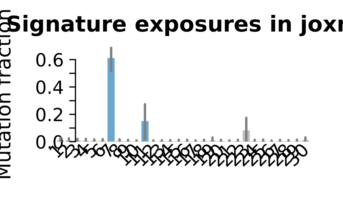
| Version | Author | Date |
|---|---|---|
| 090c1b9 | davismcc | 2018-08-24 |
....plotting kuco 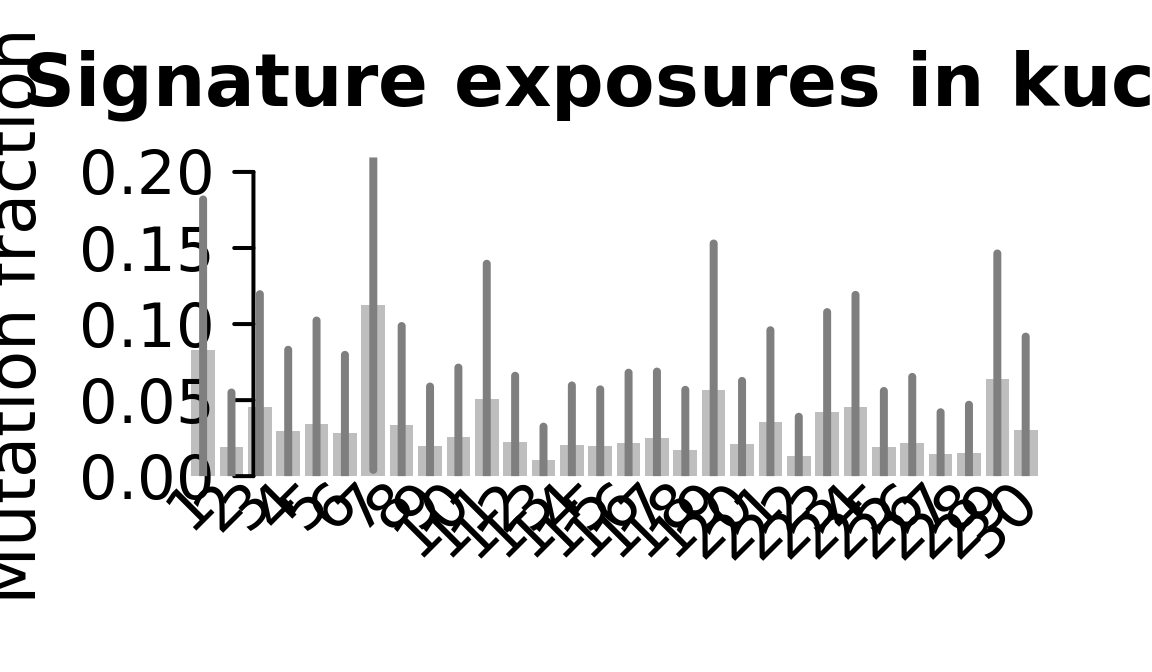
| Version | Author | Date |
|---|---|---|
| 090c1b9 | davismcc | 2018-08-24 |
....plotting laey 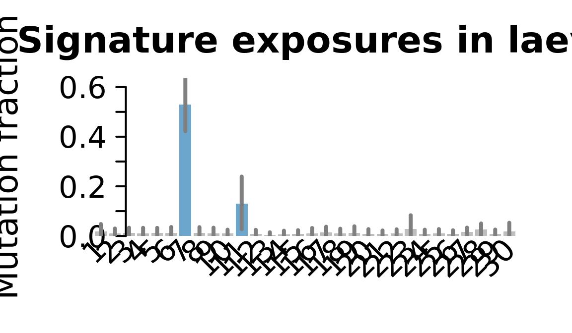
| Version | Author | Date |
|---|---|---|
| 090c1b9 | davismcc | 2018-08-24 |
....plotting lexy 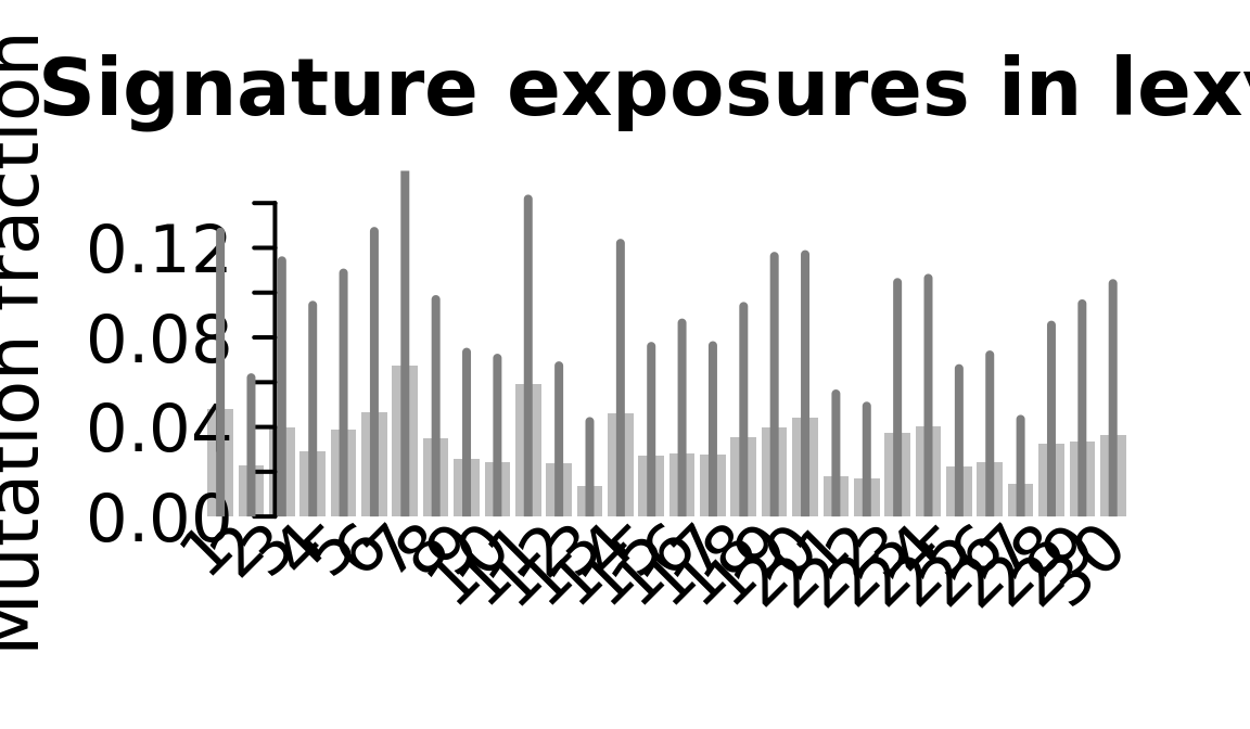
| Version | Author | Date |
|---|---|---|
| 090c1b9 | davismcc | 2018-08-24 |
....plotting naju 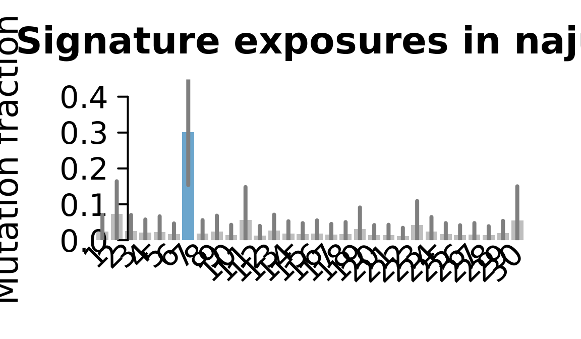
| Version | Author | Date |
|---|---|---|
| 090c1b9 | davismcc | 2018-08-24 |
....plotting nusw 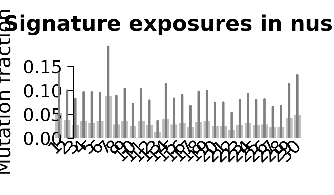
| Version | Author | Date |
|---|---|---|
| 090c1b9 | davismcc | 2018-08-24 |
....plotting oaaz 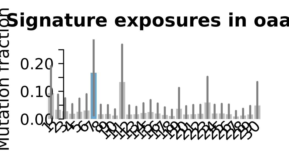
| Version | Author | Date |
|---|---|---|
| 090c1b9 | davismcc | 2018-08-24 |
....plotting oilg 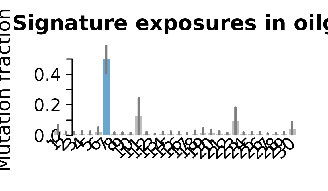
| Version | Author | Date |
|---|---|---|
| 090c1b9 | davismcc | 2018-08-24 |
....plotting pipw 
| Version | Author | Date |
|---|---|---|
| 090c1b9 | davismcc | 2018-08-24 |
....plotting puie 
| Version | Author | Date |
|---|---|---|
| 090c1b9 | davismcc | 2018-08-24 |
....plotting qayj 
| Version | Author | Date |
|---|---|---|
| 090c1b9 | davismcc | 2018-08-24 |
....plotting qolg 
| Version | Author | Date |
|---|---|---|
| 090c1b9 | davismcc | 2018-08-24 |
....plotting qonc 
| Version | Author | Date |
|---|---|---|
| 090c1b9 | davismcc | 2018-08-24 |
....plotting rozh 
| Version | Author | Date |
|---|---|---|
| 090c1b9 | davismcc | 2018-08-24 |
....plotting sehl 
| Version | Author | Date |
|---|---|---|
| 090c1b9 | davismcc | 2018-08-24 |
....plotting ualf 
| Version | Author | Date |
|---|---|---|
| 090c1b9 | davismcc | 2018-08-24 |
....plotting vass 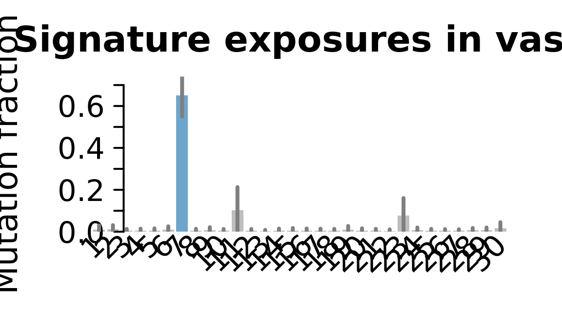
| Version | Author | Date |
|---|---|---|
| 090c1b9 | davismcc | 2018-08-24 |
....plotting vils 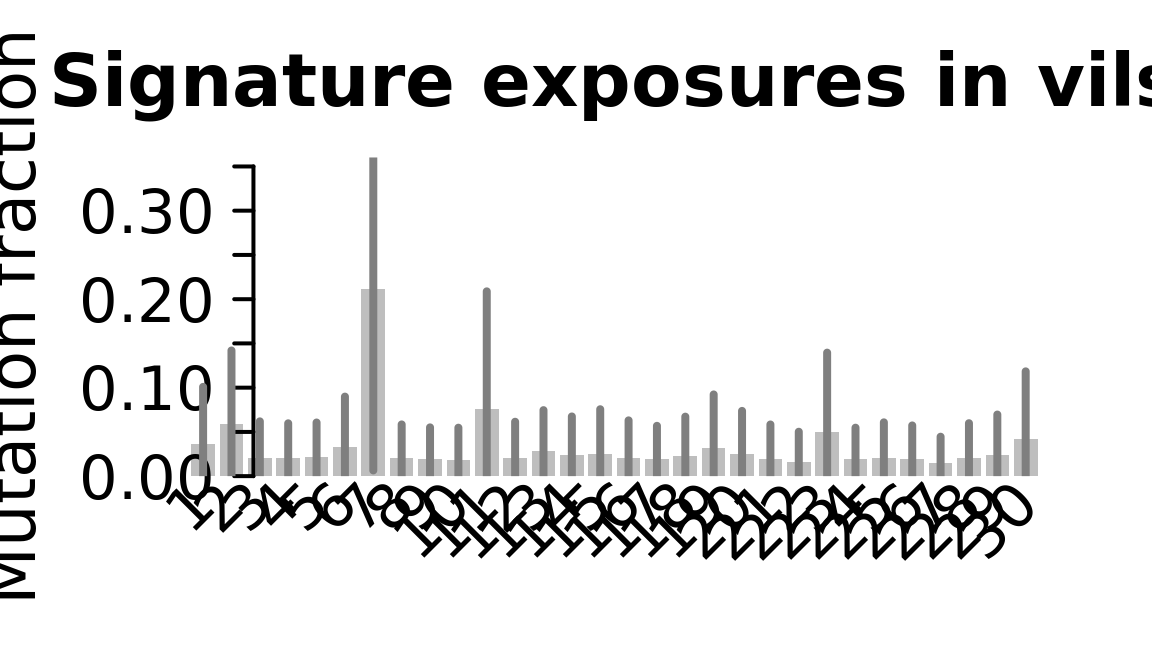
| Version | Author | Date |
|---|---|---|
| 090c1b9 | davismcc | 2018-08-24 |
....plotting vuna 
| Version | Author | Date |
|---|---|---|
| 090c1b9 | davismcc | 2018-08-24 |
....plotting wahn 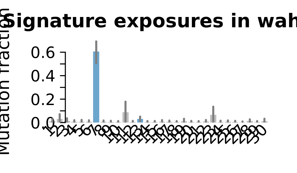
| Version | Author | Date |
|---|---|---|
| 090c1b9 | davismcc | 2018-08-24 |
....plotting wetu 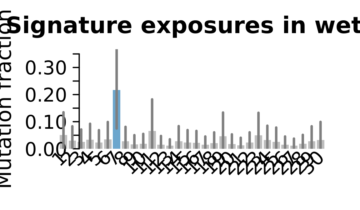
| Version | Author | Date |
|---|---|---|
| 090c1b9 | davismcc | 2018-08-24 |
....plotting xugn 
| Version | Author | Date |
|---|---|---|
| 090c1b9 | davismcc | 2018-08-24 |
....plotting zoxy 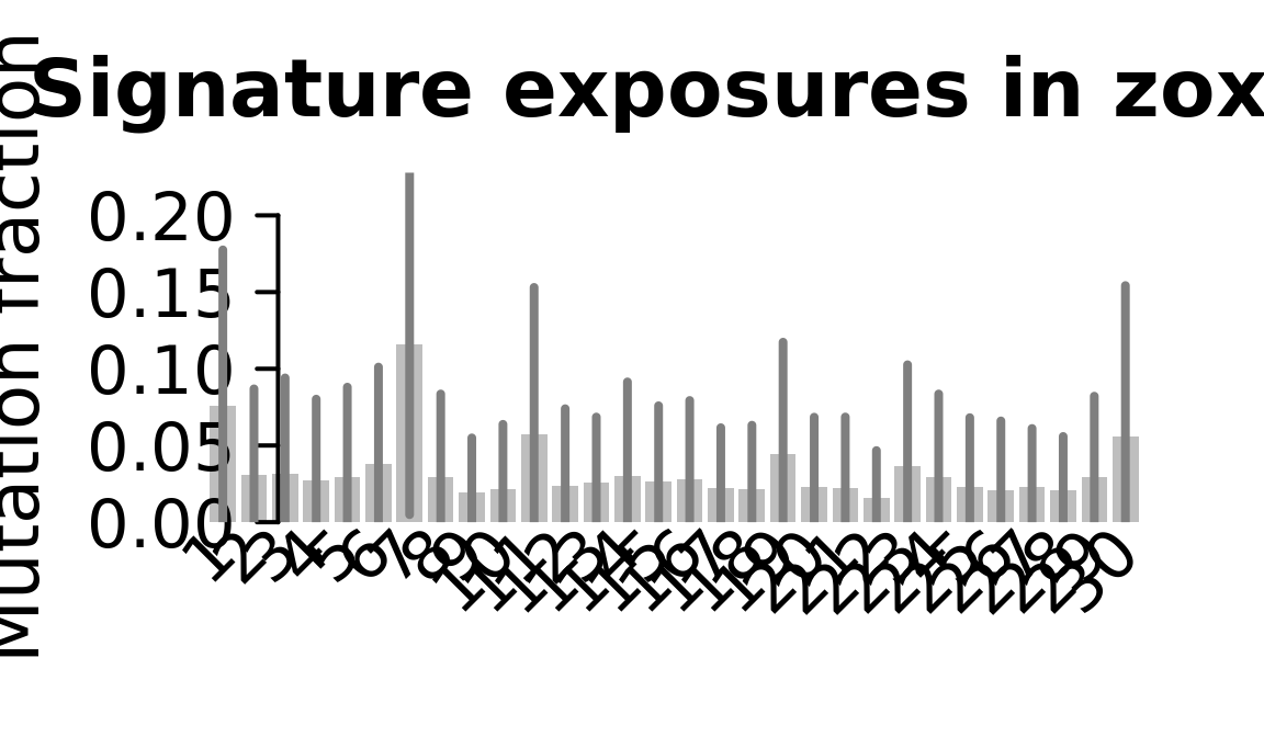
| Version | Author | Date |
|---|---|---|
| 090c1b9 | davismcc | 2018-08-24 |
Retrieve exposures for a given signal. Specifically, we will look an highest posterior density (HPD) intervals and mean exposures for Signature 7 (UV) and Signature 11, the only two that are significant across multiple lines. We add this information to the donor_info dataframe.
get_signature_df <- function(exposures, samples, signature) {
  signature_mat_mean <- matrix(NA, nrow = length(samples), 30)
  for (i in 1:length(samples)) {
    signature_mat_mean[i,] <- as.numeric(exposures[[i]]$mean)
  }
  rownames(signature_mat_mean) <- samples
  colnames(signature_mat_mean) <- colnames(exposures[[i]]$mean)
  signature_mat_lower90 <- matrix(NA, nrow = length(samples), 30)
  for (i in 1:length(samples)) {
    signature_mat_lower90[i,] <- as.numeric(exposures[[i]]$lower_90)
  }
  rownames(signature_mat_lower90) <- samples
  colnames(signature_mat_lower90) <- colnames(exposures[[i]]$lower_90)
  signature_mat_upper90 <- matrix(NA, nrow = length(samples), 30)
  for (i in 1:length(samples)) {
    signature_mat_upper90[i,] <- as.numeric(exposures[[i]]$upper_90)
  }
  rownames(signature_mat_upper90) <- samples
  colnames(signature_mat_upper90) <- colnames(exposures[[i]]$upper_90)
  signature_df <- cbind(
    as.data.frame(signature_mat_mean[,signature]),
    as.data.frame(signature_mat_lower90[,signature]),
    as.data.frame(signature_mat_upper90[,signature]))
  colnames(signature_df) <- c(paste0("Sig",signature,"_mean"),
                              paste0("Sig",signature,"_lower"),
                              paste0("Sig",signature,"_upper"))
  signature_df$donor <- rownames(signature_df)
  signature_df
}

## Get lower, mean and upper values for signatures 7 & 11
sig7_df <- get_signature_df(exposures, mutation_donors, 7)
sig11_df <- get_signature_df(exposures, mutation_donors, 11)

## Add Sigs 7/11 to donor info table
sig_subset_df <- merge(sig7_df,sig11_df, by = "donor")
sig_subset_df_means <- sig_subset_df[,c(1,grep("mean", colnames(sig_subset_df)))]
sig_subset_df_means_melt <- reshape2::melt(sig_subset_df_means)
sig_subset_df_means_melt$signature <- substr(sig_subset_df_means_melt$variable, 1, 5)
sig_subset_df_means_melt <- sig_subset_df_means_melt[,c("donor", "signature", "value")]

colnames(sig_subset_df)[1] <- "donor_short"
donor_info <- merge(donor_info, sig_subset_df, by = "donor_short")
Expression data and cell assignments
Original Cardelino cell assignments
Read in annotated SingleCellExperiment (SCE) objects and create a list of SCE objects containing all cells used for analysis and their assignment (using cardelino) to clones identified with Canopy from whole-exome sequencing data.
params <- list()
params$callset <- "filt_lenient.cell_coverage_sites"
fls <- list.files("data/sces")
fls <- fls[grepl(paste0("assignments.", params$callset), fls)]
donors <- gsub(".*ce_([a-z]+)_.*assignments.filt.*", "\\1", fls)
sce_unst_list <- list()
for (don in donors) {
    sce_unst_list[[don]] <- readRDS(file.path("data/sces",
        paste0("sce_", don, "_with_clone_assignments.", params$callset, ".rds")))
    cat(paste("reading", don, ":   ", ncol(sce_unst_list[[don]]), "cells.\n"))
}
reading euts : 79 cells.
reading fawm : 53 cells.
reading feec : 75 cells.
reading fikt : 39 cells.
reading garx : 70 cells.
reading gesg : 105 cells.
reading heja : 50 cells.
reading hipn : 62 cells.
reading ieki : 58 cells.
reading joxm : 79 cells.
reading kuco : 48 cells.
reading laey : 55 cells.
reading lexy : 63 cells.
reading naju : 44 cells.
reading nusw : 60 cells.
reading oaaz : 38 cells.
reading oilg : 90 cells.
reading pipw : 107 cells.
reading puie : 41 cells.
reading qayj : 97 cells.
reading qolg : 36 cells.
reading qonc : 58 cells.
reading rozh : 91 cells.
reading sehl : 30 cells.
reading ualf : 89 cells.
reading vass : 37 cells.
reading vils : 37 cells.
reading vuna : 71 cells.
reading wahn : 82 cells.
reading wetu : 77 cells.
reading xugn : 35 cells.
reading zoxy : 88 cells.## Calculate single cell data metrics
sc_metrics_summary <- list()
sc_metrics_summary_df <- data.frame()
for (don in donors) {
sc_metrics_summary[[don]]$num_unst_cells <- ncol(sce_unst_list[[don]])
sc_metrics_summary[[don]]$num_assignable <- sum(sce_unst_list[[don]]$assignable)
sc_metrics_summary[[don]]$num_unassignable <-
(sc_metrics_summary[[don]]$num_unst_cells -
sc_metrics_summary[[don]]$num_assignable)
sc_metrics_summary[[don]]$num_clones_with_cells <-
length(unique(sce_unst_list[[don]]$assigned[
which(sce_unst_list[[don]]$assigned != "unassigned")]))
sc_metrics_summary[[don]]$donor <- don
sc_metrics_summary_df <-
rbind(sc_metrics_summary_df, as.data.frame(sc_metrics_summary[[don]]))
}
colnames(sc_metrics_summary_df) <- c("total_unst_cells", "assigned_unst_cells",
"unassigned_unst_cells",
"num_clones_with_cells", "donor_short")
## Merge with donor info table
donor_info <- merge(donor_info, sc_metrics_summary_df, by = "donor_short",
all.x = TRUE)
donor_info$percent_assigned_cells <-
donor_info$assigned_unst_cells / donor_info$total_unst_cellsCanopy clone inference information
First, we read in the canopy output for each line we analyse.
canopy_files <- list.files("data/canopy")
canopy_files <- canopy_files[grepl(params$callset, canopy_files)]
canopy_list <- list()
for (don in donors) {
  canopy_list[[don]] <- readRDS(
    file.path("data/canopy",
              paste0("canopy_results.", don, ".", params$callset, ".rds")))
}
Second, summarise the number of mutations for each clone, for each line. Form these results into a dataframe.
clone_mut_list <- list()
for (don in donors) {
  cat(paste("summarising clones and mutations for", don, '\n'))
  clone_mut_list[[don]] <- colSums(canopy_list[[don]]$tree$Z)
  cat(colSums(canopy_list[[don]]$tree$Z))
  cat('\n')
}
summarising clones and mutations for euts
0 39 29
summarising clones and mutations for fawm
0 17 16
summarising clones and mutations for feec
0 19 9 6
summarising clones and mutations for fikt
0 13 23
summarising clones and mutations for garx
0 79 57
summarising clones and mutations for gesg
0 37 23
summarising clones and mutations for heja
0 16 20
summarising clones and mutations for hipn
0 8 8
summarising clones and mutations for ieki
0 7 10
summarising clones and mutations for joxm
0 41 98
summarising clones and mutations for kuco
0 9
summarising clones and mutations for laey
0 45 49
summarising clones and mutations for lexy
0 9 6
summarising clones and mutations for naju
0 13
summarising clones and mutations for nusw
0 3 13
summarising clones and mutations for oaaz
0 17 19
summarising clones and mutations for oilg
0 2 37
summarising clones and mutations for pipw
0 34 36
summarising clones and mutations for puie
0 13 15
summarising clones and mutations for qayj
0 11 7
summarising clones and mutations for qolg
0 23
summarising clones and mutations for qonc
0 17 7
summarising clones and mutations for rozh
0 11 10 12
summarising clones and mutations for sehl
0 2 11 23
summarising clones and mutations for ualf
0 29 39
summarising clones and mutations for vass
0 98 35
summarising clones and mutations for vils
0 1 2 8
summarising clones and mutations for vuna
0 33
summarising clones and mutations for wahn
0 52 114
summarising clones and mutations for wetu
0 8 17
summarising clones and mutations for xugn
0 16 12
summarising clones and mutations for zoxy
0 14 8clone_mut_df <- data.frame(clone1 = numeric(), clone2 = numeric(),
clone3 = numeric(), clone4 = numeric())
for (i in 1:length(donors)) {
num_clones <- length(clone_mut_list[[i]])
num_NAs <- 4 - num_clones
temp_row <- c(clone_mut_list[[i]], rep(NA, num_NAs))
clone_mut_df[i,] <- temp_row
}
rownames(clone_mut_df) <- donors
clone_mut_df$donor_short <- donorsNext, summarise the number of unique mutations tagging each clone identified by Canopy (that is, the number of variants for each clone that distinguish it from other clones in the line). Produce a dataframe with this information as well.
clone_mut_unique_list <- list()
for (don in donors) {
        cat(paste("summarising clones and mutations for", don, '\n'))
        clone_mut_unique_list[[don]] <-
          colSums(canopy_list[[don]]$tree$Z[
            (rowSums(canopy_list[[don]]$tree$Z) == 1),])
        cat(colSums(canopy_list[[don]]$tree$Z[
          (rowSums(canopy_list[[don]]$tree$Z) == 1),]))
        cat('\n')
}
summarising clones and mutations for euts
0 20 10
summarising clones and mutations for fawm
0 3 2
summarising clones and mutations for feec
0 16 4 1
summarising clones and mutations for fikt
0 3 13
summarising clones and mutations for garx
0 41 19
summarising clones and mutations for gesg
0 20 6
summarising clones and mutations for heja
0 8 12
summarising clones and mutations for hipn
0 6 6
summarising clones and mutations for ieki
0 6 9
summarising clones and mutations for joxm
0 14 71
summarising clones and mutations for kuco
0 9
summarising clones and mutations for laey
0 16 20
summarising clones and mutations for lexy
0 5 2
summarising clones and mutations for naju
0 13
summarising clones and mutations for nusw
0 0 10
summarising clones and mutations for oaaz
0 8 10
summarising clones and mutations for oilg
0 2 37
summarising clones and mutations for pipw
0 17 19
summarising clones and mutations for puie
0 4 6
summarising clones and mutations for qayj
0 7 3
summarising clones and mutations for qolg
0 23
summarising clones and mutations for qonc
0 13 3
summarising clones and mutations for rozh
0 7 0 2
summarising clones and mutations for sehl
0 0 3 15
summarising clones and mutations for ualf
0 15 25
summarising clones and mutations for vass
0 65 2
summarising clones and mutations for vils
0 0 1 7
summarising clones and mutations for vuna
0 33
summarising clones and mutations for wahn
0 1 63
summarising clones and mutations for wetu
0 2 11
summarising clones and mutations for xugn
0 6 2
summarising clones and mutations for zoxy
0 7 1clone_mut_unique_df <- data.frame(clone1 = numeric(), clone2 = numeric(),
clone3 = numeric(),
clone4 = numeric(), min_unique_muts = numeric())
for (i in 1:length(donors)) {
num_clones <- length(clone_mut_unique_list[[i]])
num_NAs <- 4 - num_clones
temp_row <- c(clone_mut_unique_list[[i]], rep(NA, num_NAs),
min(clone_mut_unique_list[[i]][2:num_clones]))
clone_mut_unique_df[i,] <- temp_row
}
rownames(clone_mut_df) <- donors
clone_mut_df$donor_short <- donors
rownames(clone_mut_unique_df) <- donors
clone_mut_unique_df$donor_short <- donors
donor_info <- merge(donor_info, clone_mut_unique_df, by = "donor_short", all.x = T)Finally, calculate the minimum Hamming distance between pairs of clones for each line. In general, assignment of cells to clones will be easier/more successful for lines with larger numbers of variants distinguishes between clones (that is, a high minimum Hamming distance).
We add all of this information to the donor_info dataframe and then have the data prepared to make some overview plots across lines.
## Calculate Hamming distance
clone_mut_list_hamming <- list()
for (don in donors) {
  Config <- canopy_list[[don]]$tree$Z
  unique_sites_paired <- c()
  for (i in seq_len(ncol(Config) - 1)) {
    for (j in seq(i + 1, ncol(Config))) {
      n_sites <- sum(rowSums(Config[, c(i,j)]) == 1)
      unique_sites_paired <- c(unique_sites_paired, n_sites)
    }
  }
  clone_mut_list_hamming[[don]] <- unique_sites_paired
  cat("....hamming distances for ", don, ": ", unique_sites_paired, "\n")
}
....hamming distances for euts : 39 29 30
....hamming distances for fawm : 17 16 5
....hamming distances for feec : 19 9 6 22 19 5
....hamming distances for fikt : 13 23 16
....hamming distances for garx : 79 57 60
....hamming distances for gesg : 37 23 26
....hamming distances for heja : 16 20 20
....hamming distances for hipn : 8 8 12
....hamming distances for ieki : 7 10 15
....hamming distances for joxm : 41 98 85
....hamming distances for kuco : 9
....hamming distances for laey : 45 49 36
....hamming distances for lexy : 9 6 7
....hamming distances for naju : 13
....hamming distances for nusw : 3 13 10
....hamming distances for oaaz : 17 19 18
....hamming distances for oilg : 2 37 39
....hamming distances for pipw : 34 36 36
....hamming distances for puie : 13 15 10
....hamming distances for qayj : 11 7 10
....hamming distances for qolg : 23
....hamming distances for qonc : 17 7 16
....hamming distances for rozh : 11 10 12 13 15 2
....hamming distances for sehl : 2 11 23 9 21 18
....hamming distances for ualf : 29 39 40
....hamming distances for vass : 98 35 67
....hamming distances for vils : 1 2 8 1 7 8
....hamming distances for vuna : 33
....hamming distances for wahn : 52 114 64
....hamming distances for wetu : 8 17 13
....hamming distances for xugn : 16 12 8
....hamming distances for zoxy : 14 8 8 min_hamming_distance <- data.frame("donor_short" = donors,
"min_hamming_dist" = 0)
for (i in 1:length(donors)) {
min_hamming_distance$min_hamming_dist[i] <- min(clone_mut_list_hamming[[i]])
}
donor_info <- merge(donor_info, min_hamming_distance, by = "donor_short",
all.x = TRUE)
## Number of clones
donor_info$num_clones_total <- 0
for (i in donors) {
num_clones <- length(clone_mut_unique_list[[i]])
donor_info$num_clones_total[which(donor_info$donor_short == i)] <- num_clones
}Plot line metrics
We make a large combined plot stitching together individual plots showing:
- donor age;
- number of somatic mutations;
- signature 7 (UV) exposure;
- probablility of selection (Williams et al, 2018); and
- number of mutations per clone
for each line.
donor_info_filt <- donor_info[which(donor_info$donor_short %in% donors), ]
donor_filt_order <- dplyr::arrange(donor_info_filt, desc(num_mutations))
donor_filt_order <- donor_filt_order$donor_short
rownames(donor_info_filt) <- donor_info_filt$donor_short

# Plot age
selected_vars <- c("donor_short", "age_decade")
donor_info_filt_melt <- reshape2::melt(donor_info_filt[,selected_vars],
                                       "donor_short")
donor_info_filt_melt <- donor_info_filt[,selected_vars]

age_plot_filt <- ggplot(
  donor_info_filt_melt,
  aes(x = "Age", y = factor(donor_short, levels = rev(donor_filt_order)),
      fill = age_decade)) +
  geom_tile() +
  labs(x = "", y = "Donor", fill = "") +
  scale_fill_manual(values = rev(c(magma(8)[-c(1,8)])))  +
  guides(fill = guide_legend(nrow = 3,byrow = TRUE)) +
  theme(axis.text.x = element_text(size = 32, face = "plain"),
        axis.line = element_blank(),
        legend.position = "top", legend.direction = "horizontal",
        legend.text = element_text(size = 28, face = "plain"),
        legend.key.size = unit(0.3,"in"),
        axis.ticks.x = element_blank(),
        legend.margin = margin(unit(0.01, "cm")),
        axis.text.y = element_text(size = 30, face = "plain"),
        axis.title.y = element_text(size = 36, face = "plain"),
        axis.title.x = element_text(size = 36, face = "plain"))

# Plot number of mutations
selected_vars <- c("donor_short", "num_mutations")
donor_info_filt_melt <- reshape2::melt(donor_info_filt[,selected_vars],
                                       "donor_short")
num_mut_plot_filt <- ggplot(
  donor_info_filt_melt,
  aes(x = value, y = factor(donor_short, levels = rev(donor_filt_order)))) +
  geom_point(size = 4, alpha = 0.7) +
  scale_shape_manual(values = c(4, 19)) +
  scale_x_log10(breaks = c(50, 100, 500)) +
  theme_bw(16) +
  ggtitle(" ") +
  labs(x = "Number of mutations", y = "") +
  theme(axis.text.y = element_blank(),
        axis.ticks.y = element_blank(),
        axis.line = element_blank(),
        legend.position = "top",
        axis.text.x = element_text(size = 32, face = "plain"),
        title = element_text(colour="black",size = 30, face = "plain"),
        axis.title.x = element_text(size = 36, face = "plain"))

# Plot signature 7
donor_info_filt_melt <- reshape2::melt(
  donor_info_filt[,c(1,grep("Sig7_mean",colnames(donor_info_filt)))])
donor_info_filt_melt$signature <- substr(donor_info_filt_melt$variable, 1, 5)
donor_info_filt_melt <-
  donor_info_filt_melt[, c("donor_short", "signature", "value")]
sig_decomp_plot_filt <- ggplot(
  donor_info_filt_melt,
  aes(y = value, x = factor(donor_short, levels = rev(donor_filt_order)),
      fill = factor(signature))) +
  geom_bar(stat = "identity") +
  coord_flip() +
  scale_fill_manual(values = rev(c(magma(10)[-c(1,10)]))) +
  theme_bw(16) +
  ggtitle(" ") +
  labs(x = "",y = "Signature 7 exposure", fill = "") +
  theme(axis.text.y = element_blank(),
        axis.ticks.y = element_blank(),
        axis.line = element_blank(),
        axis.text.x = element_text(size = 32, face = "plain"),
        title = element_text(colour = "black", size = 30, face = "plain"),
        axis.title.x = element_text(size = 36, face = "plain")) +
  guides(fill = FALSE)


# Plot selection results
donor_selection_info <- read.csv("data/p1-selection.csv", row.names=1)
donor_selection_info <- read_csv("data/p1-selection.csv")

# add missing donor (simulation failed)
donor_selection_info$ps1 <- as.numeric(donor_selection_info$ps1)
donor_selection_info$selection <- factor(donor_selection_info$selection, levels=c("neutral", "undetermined", "selected"))

selection_plot <- ggplot(donor_selection_info, aes(x=ps1, y=factor(donor, levels=rev(donor_filt_order)), colour=selection)) +
                geom_point(size = 4, alpha = 0.7) +
                coord_cartesian(xlim = c(0, 1)) +
                scale_colour_manual(values = c(neutral="#1283FF", selected="#144E7B", undetermined="#CACACA")) +
                geom_vline(xintercept=c(0.3, 0.7), colour="#808080") +
                scale_x_continuous(breaks=c(0, 0.3, 0.5, 0.7, 1.0)) +
                theme_bw(16) +
        labs(x = "Probability of Selection", y = "", colour = "Selection") +
    # guides(colour=guide_legend(title.position="top",
    #                                  title.hjust =0.5)) +
    guides(colour = guide_legend(ncol = 1)) +
        theme(axis.ticks.y = element_blank(),
        axis.line = element_blank(),
            legend.position = "top",
            legend.key.size = unit(0.3,"in"),
            axis.title.x = element_text(size = 36, face = "plain"),
            axis.text.x = element_text(size = 32, face = "plain"),
            axis.text.y = element_blank(),
            legend.justification = "center",
            legend.text = element_text(size = 28, face = "plain"),
            legend.title = element_text(size = 30, face = "plain"))


# Plot total number of mutations per clone
donor_info_filt_subset <-
  donor_info_filt[,c(1,grep("clone",colnames(donor_info_filt)))]
# Remove columns that do not relate to number of mutations per clone:
donor_info_filt_subset <- donor_info_filt_subset[,c(-2,-7)]
donor_info_filt_melt <- reshape2::melt(donor_info_filt_subset, "donor_short")
donor_info_filt_melt$variable <- substr(donor_info_filt_melt$variable, 6, 6)
num_clones_plot_filt <- ggplot(
  donor_info_filt_melt,
  aes(variable, factor(donor_short, levels = rev(donor_filt_order)))) +
  geom_tile(aes(fill = value), colour = "white") +
  scale_fill_distiller(palette = "BuPu", values = c(0,0.05,0.1,0.15,0.25,0.5,1),
                       na.value = "white", breaks = c(0,25,50,75),
                       direction = 1) +
  labs(x = "Clone", y = "", fill = "Number of mutations") +
  theme(axis.ticks.y = element_blank(),
        axis.line = element_blank(),
        legend.position = "top",
        legend.key.size = unit(0.3,"in"),
        axis.title.x = element_text(size = 36, face = "plain"),
        axis.text.x = element_text(size = 32, face = "plain"),
        axis.text.y = element_blank(),
        legend.justification = "center",
        legend.text = element_text(size = 28, face = "plain"),
        legend.title = element_text(size = 30, face = "plain"))

## Combine above plots into Fig 2a
fig_2a <- cowplot::plot_grid(age_plot_filt, num_mut_plot_filt,
                             sig_decomp_plot_filt, selection_plot, num_clones_plot_filt,
                             nrow = 1, rel_widths = c(3, 4, 4, 4, 4), align = "h",
                             axis = "t", scale =  c(1, 0.988, 0.988, 0.988))
ggsave("figures/overview_lines/overview_lines_BuPu.png",
       plot = fig_2a, width = 30, height = 14)

fig_2a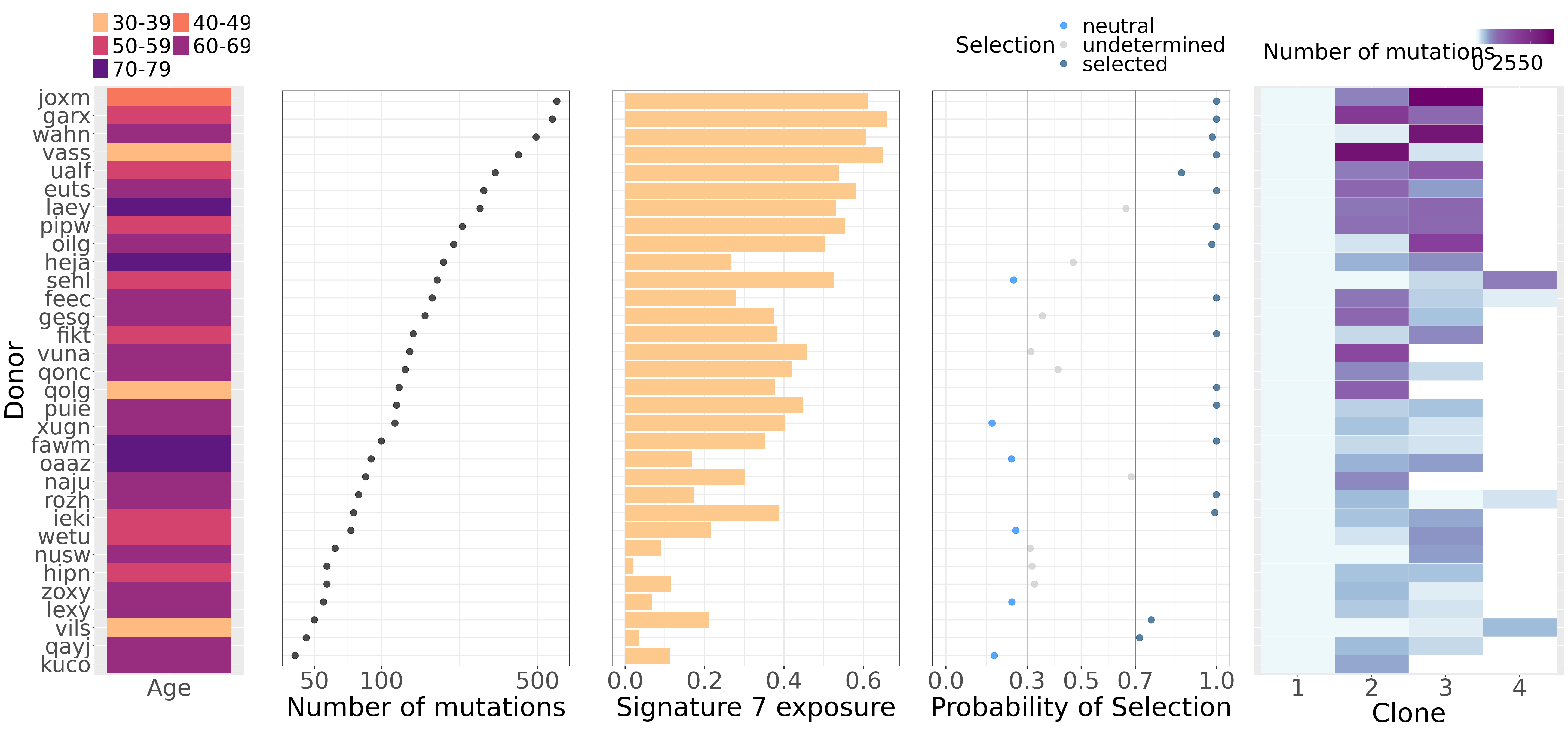
Plot cell assignment rate vs Hamming Distance
Finally, we plot the cell assignment rate (from cardelino) against the minimum Hamming distance (minimum number of variants distinguishing a pair of clones) for each line.
fig_2c_no_size <- ggplot(
  donor_info_filt,
  aes(y = as.numeric(percent_assigned_cells), x = as.numeric(min_hamming_dist),
      fill = total_unst_cells)) +
  geom_point(pch = 21, colour = "gray50", size = 4) +
  scale_shape_manual(values = c(4, 19)) +
  ylim(c(0, 1)) +
  scale_x_log10() +
  scale_fill_viridis(option = "magma") +
  ylab("Proportion cells assigned") +
  xlab("Minimum number of variants distinguishing clones") +
  labs(title = "") +
  labs(fill = "Number of cells") +
  theme_bw() +
  theme(text = element_text(size = 9,face = "bold"),
        axis.text = element_text(size = 9, face = "bold"),
        axis.title = element_text(size = 10, face = "bold"),
        plot.title = element_text(size = 9, hjust = 0.5)) +
  theme(strip.background = element_blank()) +
  theme(legend.justification = c(1,0),
        legend.position = c(1,0),
        legend.direction = "horizontal",
        legend.background = element_rect(fill = "white", linetype = 1,
                                         colour = "black", size = 0.2),
        legend.key.size = unit(0.25, "cm"))

ggsave("figures/overview_lines/cell_assignment_vs_min_hamming_dist.png",
       plot = fig_2c_no_size, width = 12, height = 12, dpi = 300, units = "cm")
fig_2c_no_size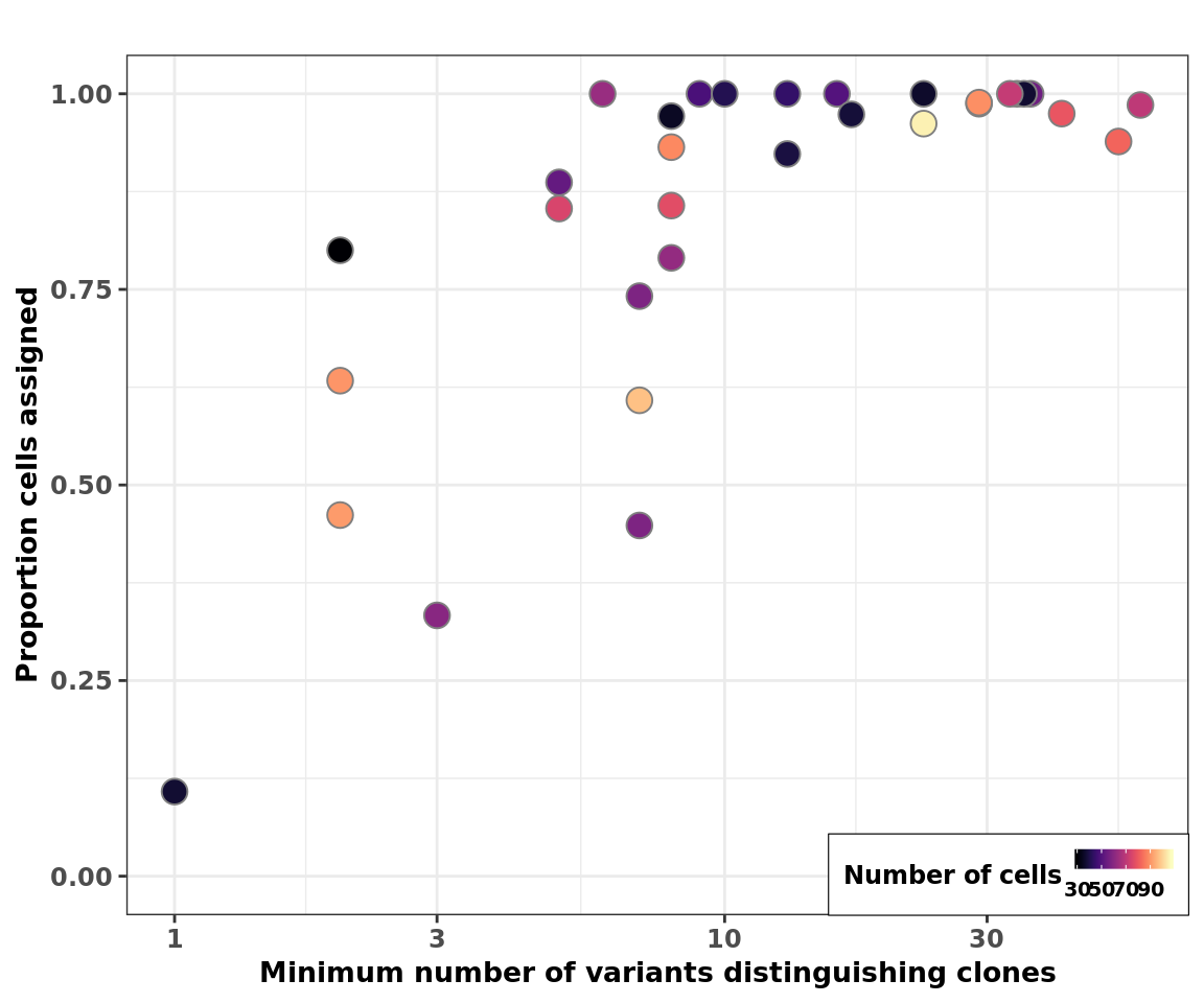
| Version | Author | Date |
|---|---|---|
| 090c1b9 | davismcc | 2018-08-24 |
Save data to file
Save the donor info dataframe to output/line_info.tsv.
─ Session info ──────────────────────────────────────────────────────────
 setting  value
 version  R version 3.6.0 (2019-04-26)
 os       Ubuntu 18.04.3 LTS
 system   x86_64, linux-gnu
 ui       X11
 language (EN)
 collate  en_AU.UTF-8
 ctype    en_AU.UTF-8
 tz       Australia/Melbourne
 date     2019-10-30

─ Packages ──────────────────────────────────────────────────────────────
 package                     * version   date       lib
 AnnotationDbi               * 1.46.1    2019-08-20 [1]
 assertthat                    0.2.1     2019-03-21 [1]
 backports                     1.1.4     2019-04-10 [1]
 beeswarm                      0.2.3     2016-04-25 [1]
 Biobase                     * 2.44.0    2019-05-02 [1]
 BiocGenerics                * 0.30.0    2019-05-02 [1]
 BiocNeighbors                 1.2.0     2019-05-02 [1]
 BiocParallel                * 1.18.1    2019-08-06 [1]
 BiocSingular                  1.0.0     2019-05-02 [1]
 Biostrings                    2.52.0    2019-05-02 [1]
 bit                           1.1-14    2018-05-29 [1]
 bit64                         0.9-7     2017-05-08 [1]
 bitops                        1.0-6     2013-08-17 [1]
 blob                          1.2.0     2019-07-09 [1]
 BSgenome                      1.52.0    2019-05-02 [1]
 BSgenome.Hsapiens.UCSC.hg19   1.4.0     2019-06-28 [1]
 callr                         3.3.2     2019-09-22 [1]
 caTools                       1.17.1.2  2019-03-06 [1]
 cli                           1.1.0     2019-03-19 [1]
 clue                          0.3-57    2019-02-25 [1]
 cluster                       2.1.0     2019-06-19 [1]
 coda                          0.19-3    2019-07-05 [1]
 codetools                     0.2-16    2018-12-24 [4]
 colorspace                    1.4-1     2019-03-18 [1]
 cowplot                     * 1.0.0     2019-07-11 [1]
 crayon                        1.3.4     2017-09-16 [1]
 DBI                           1.0.0     2018-05-02 [1]
 deconstructSigs             * 1.8.0     2016-07-29 [1]
 DelayedArray                * 0.10.0    2019-05-02 [1]
 DelayedMatrixStats            1.6.1     2019-09-08 [1]
 desc                          1.2.0     2018-05-01 [1]
 devtools                      2.2.1     2019-09-24 [1]
 digest                        0.6.21    2019-09-20 [1]
 dplyr                       * 0.8.3     2019-07-04 [1]
 dqrng                         0.2.1     2019-05-17 [1]
 dynamicTreeCut                1.63-1    2016-03-11 [1]
 edgeR                       * 3.26.8    2019-09-01 [1]
 ellipsis                      0.3.0     2019-09-20 [1]
 evaluate                      0.14      2019-05-28 [1]
 farver                        1.1.0     2018-11-20 [1]
 fs                            1.3.1     2019-05-06 [1]
 gdata                         2.18.0    2017-06-06 [1]
 GenomeInfoDb                * 1.20.0    2019-05-02 [1]
 GenomeInfoDbData              1.2.1     2019-04-30 [1]
 GenomicAlignments             1.20.1    2019-06-18 [1]
 GenomicRanges               * 1.36.1    2019-09-06 [1]
 ggbeeswarm                    0.6.0     2017-08-07 [1]
 ggforce                     * 0.3.1     2019-08-20 [1]
 ggplot2                     * 3.2.1     2019-08-10 [1]
 ggrepel                     * 0.8.1     2019-05-07 [1]
 ggridges                    * 0.5.1     2018-09-27 [1]
 git2r                         0.26.1    2019-06-29 [1]
 glue                          1.3.1     2019-03-12 [1]
 gplots                      * 3.0.1.1   2019-01-27 [1]
 gridExtra                     2.3       2017-09-09 [1]
 gtable                        0.3.0     2019-03-25 [1]
 gtools                        3.8.1     2018-06-26 [1]
 hms                           0.5.1     2019-08-23 [1]
 htmltools                     0.3.6     2017-04-28 [1]
 igraph                        1.2.4.1   2019-04-22 [1]
 inline                        0.3.15    2018-05-18 [1]
 IRanges                     * 2.18.3    2019-09-24 [1]
 irlba                         2.3.3     2019-02-05 [1]
 KernSmooth                    2.23-15   2015-06-29 [1]
 knitr                         1.25      2019-09-18 [1]
 labeling                      0.3       2014-08-23 [1]
 lattice                       0.20-38   2018-11-04 [4]
 lazyeval                      0.2.2     2019-03-15 [1]
 limma                       * 3.40.6    2019-07-26 [1]
 locfit                        1.5-9.1   2013-04-20 [1]
 loo                           2.1.0     2019-03-13 [1]
 magrittr                      1.5       2014-11-22 [1]
 MASS                          7.3-51.1  2018-11-01 [4]
 Matrix                        1.2-17    2019-03-22 [1]
 matrixStats                 * 0.55.0    2019-09-07 [1]
 memoise                       1.1.0     2017-04-21 [1]
 munsell                       0.5.0     2018-06-12 [1]
 org.Hs.eg.db                * 3.8.2     2019-05-01 [1]
 pillar                        1.4.2     2019-06-29 [1]
 pkgbuild                      1.0.5     2019-08-26 [1]
 pkgconfig                     2.0.3     2019-09-22 [1]
 pkgload                       1.0.2     2018-10-29 [1]
 plyr                          1.8.4     2016-06-08 [1]
 polyclip                      1.10-0    2019-03-14 [1]
 prettyunits                   1.0.2     2015-07-13 [1]
 processx                      3.4.1     2019-07-18 [1]
 ps                            1.3.0     2018-12-21 [1]
 purrr                         0.3.2     2019-03-15 [1]
 R6                            2.4.0     2019-02-14 [1]
 RColorBrewer                  1.1-2     2014-12-07 [1]
 Rcpp                        * 1.0.2     2019-07-25 [1]
 RCurl                         1.95-4.12 2019-03-04 [1]
 readr                       * 1.3.1     2018-12-21 [1]
 remotes                       2.1.0     2019-06-24 [1]
 reshape2                      1.4.3     2017-12-11 [1]
 rlang                         0.4.0     2019-06-25 [1]
 rmarkdown                     1.15      2019-08-21 [1]
 rprojroot                     1.3-2     2018-01-03 [1]
 Rsamtools                     2.0.1     2019-09-19 [1]
 RSQLite                       2.1.2     2019-07-24 [1]
 rstan                         2.19.2    2019-07-09 [1]
 rsvd                          1.0.2     2019-07-29 [1]
 rtracklayer                   1.44.4    2019-09-06 [1]
 S4Vectors                   * 0.22.1    2019-09-09 [1]
 scales                        1.0.0     2018-08-09 [1]
 scater                      * 1.12.2    2019-05-24 [1]
 scran                       * 1.12.1    2019-05-27 [1]
 sessioninfo                   1.1.1     2018-11-05 [1]
 sigfit                      * 1.3.2     2019-10-30 [1]
 SingleCellExperiment        * 1.6.0     2019-05-02 [1]
 StanHeaders                   2.19.0    2019-09-07 [1]
 statmod                       1.4.32    2019-05-29 [1]
 stringi                       1.4.3     2019-03-12 [1]
 stringr                       1.4.0     2019-02-10 [1]
 SummarizedExperiment        * 1.14.1    2019-07-31 [1]
 testthat                      2.2.1     2019-07-25 [1]
 tibble                        2.1.3     2019-06-06 [1]
 tidyselect                    0.2.5     2018-10-11 [1]
 tweenr                        1.0.1     2018-12-14 [1]
 usethis                       1.5.1     2019-07-04 [1]
 vctrs                         0.2.0     2019-07-05 [1]
 vipor                         0.4.5     2017-03-22 [1]
 viridis                     * 0.5.1     2018-03-29 [1]
 viridisLite                 * 0.3.0     2018-02-01 [1]
 whisker                       0.4       2019-08-28 [1]
 withr                         2.1.2     2018-03-15 [1]
 workflowr                     1.4.0     2019-06-08 [1]
 xfun                          0.9       2019-08-21 [1]
 XML                           3.98-1.20 2019-06-06 [1]
 XVector                       0.24.0    2019-05-02 [1]
 yaml                          2.2.0     2018-07-25 [1]
 zeallot                       0.1.0     2018-01-28 [1]
 zlibbioc                      1.30.0    2019-05-02 [1]
 source
 Bioconductor
 CRAN (R 3.6.0)
 CRAN (R 3.6.0)
 CRAN (R 3.6.0)
 Bioconductor
 Bioconductor
 Bioconductor
 Bioconductor
 Bioconductor
 Bioconductor
 CRAN (R 3.6.0)
 CRAN (R 3.6.0)
 CRAN (R 3.6.0)
 CRAN (R 3.6.0)
 Bioconductor
 Bioconductor
 CRAN (R 3.6.0)
 CRAN (R 3.6.0)
 CRAN (R 3.6.0)
 CRAN (R 3.6.0)
 CRAN (R 3.6.0)
 CRAN (R 3.6.0)
 CRAN (R 3.5.2)
 CRAN (R 3.6.0)
 CRAN (R 3.6.0)
 CRAN (R 3.6.0)
 CRAN (R 3.6.0)
 CRAN (R 3.6.0)
 Bioconductor
 Bioconductor
 CRAN (R 3.6.0)
 CRAN (R 3.6.0)
 CRAN (R 3.6.0)
 CRAN (R 3.6.0)
 CRAN (R 3.6.0)
 CRAN (R 3.6.0)
 Bioconductor
 CRAN (R 3.6.0)
 CRAN (R 3.6.0)
 CRAN (R 3.6.0)
 CRAN (R 3.6.0)
 CRAN (R 3.6.0)
 Bioconductor
 Bioconductor
 Bioconductor
 Bioconductor
 CRAN (R 3.6.0)
 CRAN (R 3.6.0)
 CRAN (R 3.6.0)
 CRAN (R 3.6.0)
 CRAN (R 3.6.0)
 CRAN (R 3.6.0)
 CRAN (R 3.6.0)
 CRAN (R 3.6.0)
 CRAN (R 3.6.0)
 CRAN (R 3.6.0)
 CRAN (R 3.6.0)
 CRAN (R 3.6.0)
 CRAN (R 3.6.0)
 CRAN (R 3.6.0)
 CRAN (R 3.6.0)
 Bioconductor
 CRAN (R 3.6.0)
 CRAN (R 3.6.0)
 CRAN (R 3.6.0)
 CRAN (R 3.6.0)
 CRAN (R 3.5.1)
 CRAN (R 3.6.0)
 Bioconductor
 CRAN (R 3.6.0)
 CRAN (R 3.6.0)
 CRAN (R 3.6.0)
 CRAN (R 3.5.1)
 CRAN (R 3.6.0)
 CRAN (R 3.6.0)
 CRAN (R 3.6.0)
 CRAN (R 3.6.0)
 Bioconductor
 CRAN (R 3.6.0)
 CRAN (R 3.6.0)
 CRAN (R 3.6.0)
 CRAN (R 3.6.0)
 CRAN (R 3.6.0)
 CRAN (R 3.6.0)
 CRAN (R 3.6.0)
 CRAN (R 3.6.0)
 CRAN (R 3.6.0)
 CRAN (R 3.6.0)
 CRAN (R 3.6.0)
 CRAN (R 3.6.0)
 CRAN (R 3.6.0)
 CRAN (R 3.6.0)
 CRAN (R 3.6.0)
 CRAN (R 3.6.0)
 CRAN (R 3.6.0)
 CRAN (R 3.6.0)
 CRAN (R 3.6.0)
 CRAN (R 3.6.0)
 Bioconductor
 CRAN (R 3.6.0)
 CRAN (R 3.6.0)
 CRAN (R 3.6.0)
 Bioconductor
 Bioconductor
 CRAN (R 3.6.0)
 Bioconductor
 Bioconductor
 CRAN (R 3.6.0)
 Github (kgori/sigfit@2c16353)
 Bioconductor
 CRAN (R 3.6.0)
 CRAN (R 3.6.0)
 CRAN (R 3.6.0)
 CRAN (R 3.6.0)
 Bioconductor
 CRAN (R 3.6.0)
 CRAN (R 3.6.0)
 CRAN (R 3.6.0)
 CRAN (R 3.6.0)
 CRAN (R 3.6.0)
 CRAN (R 3.6.0)
 CRAN (R 3.6.0)
 CRAN (R 3.6.0)
 CRAN (R 3.6.0)
 CRAN (R 3.6.0)
 CRAN (R 3.6.0)
 CRAN (R 3.6.0)
 CRAN (R 3.6.0)
 CRAN (R 3.6.0)
 Bioconductor
 CRAN (R 3.6.0)
 CRAN (R 3.6.0)
 Bioconductor

[1] /home/AD.SVI.EDU.AU/dmccarthy/R/x86_64-pc-linux-gnu-library/3.6
[2] /usr/local/lib/R/site-library
[3] /usr/lib/R/site-library
[4] /usr/lib/R/library